What is a DBMS and what are its uses? Describe RDBMS with examples.
DBMS (Database Management System) refers to a collection of applications or programs that allow users to **create and maintain
databases**.
Key Features:
- Provides tools or interfaces for performing various operations such as inserting, deleting, updating data into a database.
- Stores data in a more compact and secure way compared to file-based systems.
- Helps overcome problems like data inconsistency and redundancy, making database use more organized and convenient.
Examples of DBMS:
- File systems
- XML
- Windows Registry
RDBMS (Relational Database Management System):
- Introduced in the 1970s.
- Stores data in tables rather than files, improving data access efficiency.
- Supports relationships between data using keys and constraints.
Examples of RDBMS:
- MySQL
- Oracle DB
- PostgreSQL
- SQL Server
How would you define a database?
A database is an organized, consistent, and logical collection of data that can be easily updated, accessed, and managed.
Key Characteristics:
- Mostly consists of tables or objects created using commands.
- Contains records and fields structured for efficient access.
Components:
Tuple (Row):
- Represents a single record in a table.
Attribute (Column):
- Contains data about a specific aspect of the table.
Data Retrieval:
- DBMS retrieves data from the database based on user queries.
- Provides structured access for both interactive and programmatic use.
What problems are associated with traditional file-based systems that make DBMS a preferable option?
Traditional file-based systems suffer from several limitations that DBMS effectively addresses:
Problems with File-Based Systems:
No Indexing:
- Lack indexing, forcing full scans of pages.
- Makes data access slow and tedious.
Redundancy and Inconsistency:
- Duplicate data scattered across files.
- Updates become difficult — same data needs updating in multiple places.
Unorganized Data:
- Data is unorganized, complicating access and retrieval.
No Concurrency Control:
- Lack of concurrency control causes entire pages to be locked during operations.
- Multiple users cannot access data simultaneously.
How DBMS Solves These Problems:
- Supports multiple concurrent transactions.
- Enforces integrity checks.
- Provides data isolation.
- Ensures atomicity of operations.
- Implements security through access control.
Can you explain some benefits of using a DBMS?
DBMS provides several significant advantages over traditional data storage approaches:
Data Sharing:
- Enables multiple users to access data simultaneously.
- Allows quick response to changes in data.
Integrity Constraints:
- Organizes data in a refined manner.
- Enforces rules to maintain accuracy and consistency.
Controlling Redundancy:
- Integrates all data into one database, eliminating duplication.
- Reduces storage waste and inconsistency.
Data Independence:
- Allows structural changes without affecting application programs.
- Provides logical and physical data independence.
Backup and Recovery:
- Automates data backup and restoration processes.
- Protects against data loss due to system failures.
Data Security:
- Uses authentication and encryption to protect sensitive data.
- Implements role-based access control for users.
What different types of languages are available in DBMS?
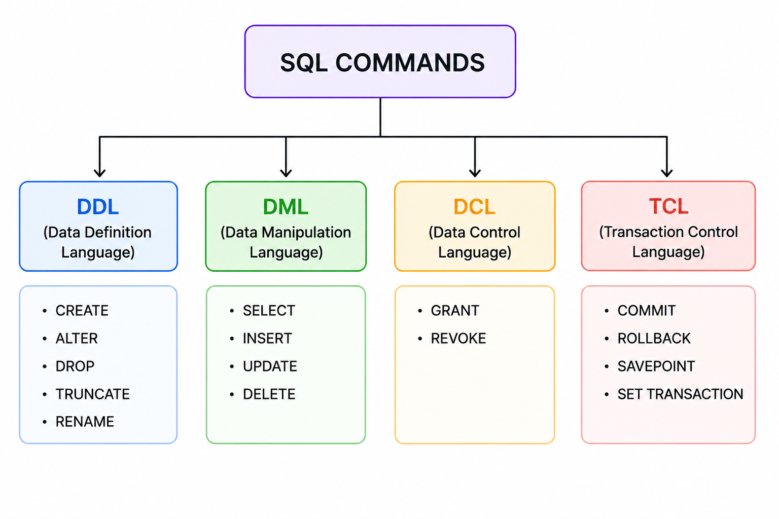
DBMS provides four main categories of languages for different database operations:
DDL (Data Definition Language):
- Used for defining database structures.
- Commands: `CREATE`, `ALTER`, `DROP`, `TRUNCATE`, `RENAME`.
- Example: `CREATE TABLE Student (id INT, name VARCHAR(50));`
DML (Data Manipulation Language):
- Used for data manipulation.
- Commands: `SELECT`, `UPDATE`, `INSERT`, `DELETE`.
- Example: `SELECT * FROM Student WHERE age > 18;`
DCL (Data Control Language):
- Used for user permissions and access control.
- Commands: `GRANT`, `REVOKE`.
- Example: `GRANT SELECT ON Student TO user1;`
TCL (Transaction Control Language):
- Used for handling transactions.
- Commands: `COMMIT`, `ROLLBACK`, `SAVEPOINT`.
- Example: `COMMIT;` to save changes permanently.
What do ACID properties mean in the context of DBMS?
ACID properties in DBMS guarantee safe and reliable data sharing during transactions.
Atomicity:
- Ensures transactions are fully completed or not executed at all.
- All operations within a transaction succeed, or none do (all-or-nothing).
Consistency:
- Keeps data valid before and after transactions.
- Database remains in a consistent state — all integrity constraints are maintained.
Isolation:
- Ensures transactions run independently without interference.
- Concurrent transactions appear as if they executed serially.
Durability:
- Ensures data persists after system failures or restarts.
- Once a transaction is committed, changes are permanent even if the system crashes.
Why ACID Matters:
- Critical for banking, e-commerce, and financial systems.
- Prevents data corruption from concurrent access or system crashes.
- Foundation of reliable transactional databases.
Are NULL values in a database equivalent to blank spaces or zeros?
NULL values are NOT equivalent to zeros or blank spaces — they have distinct meaning in databases.
What NULL Represents:
- Unknown data.
- Unavailable data.
- Inapplicable data.
What NULL is NOT:
- NULL is not a character like a blank space.
- NULL is not a numerical value like zero.
Example:
| Field | Value | Meaning |
|---|---|---|
| number_of_courses | NULL | Value is unknown — we don't know how many courses |
| number_of_courses | 0 | We know the student has taken zero courses |
| number_of_courses | "" (blank) | Empty string — different from NULL |
Important Behaviors:
- NULL cannot be compared using `=` operator — use `IS NULL` or `IS NOT NULL`.
- Arithmetic with NULL returns NULL (e.g., `5 + NULL = NULL`).
- Aggregate functions like `COUNT(column)` ignore NULL values.
What is a Database Management System (DBMS)?
A DBMS (Database Management System) is software used for managing and organizing databases.
Core Purpose:
- Provides an interface to store, retrieve, and update data.
- Ensures data integrity, security, and concurrency control.
Key Functions:
Data Storage:
- Stores data efficiently in a structured format.
Data Retrieval:
- Provides query languages (like SQL) to access stored data.
Data Manipulation:
- Supports inserting, updating, and deleting records.
Data Integrity:
- Enforces constraints to maintain data correctness.
Security:
- Controls user access through authentication and authorization.
Concurrency Control:
- Allows multiple users to access data simultaneously without conflicts.
Popular DBMS Examples:
- MySQL — open-source, widely used in web applications.
- PostgreSQL — advanced open-source RDBMS.
- Oracle — enterprise-level commercial DBMS.
- SQL Server — Microsoft's enterprise DBMS.
What advantages does using a DBMS provide?
DBMS offers several key benefits that make it superior to traditional file systems:
Data Integrity:
- Ensures accurate and reliable data through constraints.
- Maintains correctness across all transactions.
Data Security:
- Controls user access through authentication and permissions.
- Protects sensitive data from unauthorized access.
Efficient Data Retrieval:
- Uses optimized queries and indexing for fast access.
- Query optimizer chooses the best execution plan.
Reduced Redundancy:
- Eliminates duplicate data through normalization.
- Saves storage space and prevents inconsistency.
Backup and Recovery:
- Provides built-in mechanisms for regular backups.
- Enables recovery from system failures or data corruption.
Concurrent Access:
- Supports multiple simultaneous users without conflicts.
- Uses locking and isolation to maintain data consistency.
Data Independence:
- Separates physical storage from logical data structure.
- Application code doesn't break when storage changes.
How does DBMS differ from RDBMS?
DBMS vs RDBMS — Key Differences:
Data Storage Format:
- DBMS: Stores data as files or non-relational formats without enforced relationships.
- RDBMS: Stores data in tables with rows and columns based on relational model.
Relationships:
- DBMS: Does not enforce relationships between data.
- RDBMS: Supports relationships using foreign keys and primary keys.
Integrity Constraints:
- DBMS: Does not enforce integrity constraints strictly.
- RDBMS: Strictly enforces integrity constraints like NOT NULL, UNIQUE, etc.
Normalization:
- DBMS: Does not support normalization concepts.
- RDBMS: Supports normalization to reduce redundancy.
ACID Properties:
- DBMS: May not follow ACID properties.
- RDBMS: Strictly follows ACID properties for transactions.
Examples:
DBMS Examples:
- Microsoft Access
- XML databases
- File-based systems
RDBMS Examples:
- MySQL
- Oracle
- SQL Server
- PostgreSQL
What are the various types of DBMS?
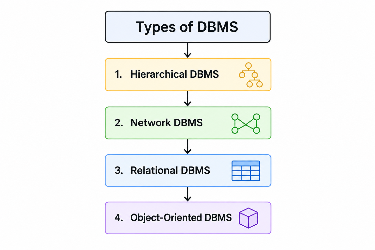
There are four main types of Database Management Systems:
Hierarchical DBMS:
- Organizes data in a tree-like parent-child structure.
- Each child has only one parent.
- Fast for one-to-many relationships.
- Example: IBM IMS (Information Management System).
Network DBMS:
- Uses a graph structure allowing many-to-many relationships.
- More flexible than hierarchical — child can have multiple parents.
- Example: IDS (Integrated Data Store), IDMS.
Relational DBMS (RDBMS):
- Table-based structure with rows and columns.
- Supports SQL for queries and data manipulation.
- Most widely used type today.
- Examples: MySQL, PostgreSQL, Oracle, SQL Server.
Object-Oriented DBMS (OODBMS):
- Stores data as objects like in object-oriented programming.
- Supports inheritance, encapsulation, and polymorphism.
- Useful for complex data types.
- Example: ObjectDB, db4o.
Modern Trend:
- Relational DBMS dominates the market.
- NoSQL databases (MongoDB, Cassandra) are emerging for big data.
What does the term relation mean in DBMS?
A relation in DBMS is a table consisting of rows and columns.
Structure of a Relation:
Rows (Tuples):
- Each row represents a single record or entity instance.
- Contains values for all attributes of the entity.
Columns (Attributes):
- Each column represents an attribute or property describing the entity.
- Has a specific data type (INT, VARCHAR, DATE, etc.).
Schema:
- Relations are defined by schemas specifying the attributes.
- Schema defines the structure — column names, data types, and constraints.
Example:
```
STUDENT Relation:
+---------+--------+-----+----------+
| Roll_No | Name | Age | Branch |
+---------+--------+-----+----------+
| 101 | Alice | 20 | CSE |
| 102 | Bob | 21 | ECE |
| 103 | Carol | 19 | CSE |
+---------+--------+-----+----------+
```
Key Properties of Relations:
- Each row is unique — no two rows are identical.
- Order of rows does not matter.
- Order of columns does not matter (referenced by name).
- All values in a column are of the same data type.
How is a table defined in DBMS?
A table in DBMS organizes data into rows and columns — the fundamental structure for storing data.
Components of a Table:
Rows:
- Each row represents a single entity or record.
- Contains values for all defined columns.
Columns:
- Each column represents attributes of the entity.
- Has a specific name and data type.
Creating a Table:
```sql
CREATE TABLE Student (
Roll_No INT PRIMARY KEY,
Name VARCHAR(50) NOT NULL,
Age INT CHECK (Age >= 18),
Branch VARCHAR(20)
);
```
Key Properties:
- Tables are the fundamental structure for storing data in RDBMS.
- Each table represents a single entity type (e.g., Student, Employee).
- Tables can be linked through keys (Primary, Foreign).
- Constraints ensure data integrity at the table level.
Table Operations:
- CREATE — defines a new table.
- ALTER — modifies table structure.
- DROP — removes the table.
- TRUNCATE — removes all rows but keeps structure.
What do rows and columns represent in a DBMS?
In DBMS, rows and columns form the basic structure of tables — each serving a distinct purpose.
Rows (Tuples):
- Represent individual records in the table.
- Contain values for each attribute (column).
- Each row is a single instance of the entity.
- Example: One row in a Student table represents one student.
Columns (Attributes):
- Define properties or characteristics of the data.
- Each column has a specific data type (INT, VARCHAR, DATE, BOOLEAN, etc.).
- Have constraints like NOT NULL, UNIQUE, PRIMARY KEY.
Example:
```
EMPLOYEE Table:
+--------+---------+--------+----------+
| Emp_ID | Name | Salary | Dept | ← Columns (Attributes)
+--------+---------+--------+----------+
| 1 | Alice | 50000 | HR | ← Row (Tuple/Record)
| 2 | Bob | 60000 | IT | ← Row (Tuple/Record)
| 3 | Charlie | 55000 | Finance | ← Row (Tuple/Record)
+--------+---------+--------+----------+
```
Key Differences:
| Aspect | Rows | Columns |
|---|---|---|
| Represents | Individual records | Attributes/properties |
| Other names | Tuples, Records | Fields, Attributes |
| Number | Variable (grows with data) | Fixed (defined in schema) |
| Order | Doesn't matter | Doesn't matter (named access) |
What are the main components of a DBMS?
The primary components of a DBMS work together to manage data effectively:
Database Engine:
- Manages data storage and retrieval.
- Core component handling input/output operations.
- Executes queries and returns results.
Database Schema:
- Defines the structure of the database.
- Includes tables, columns, data types, relationships, and constraints.
- Acts as a blueprint for data organization.
Query Processor:
- Interprets and executes SQL queries.
- Includes:
- Parser — analyzes query syntax.
- Optimizer — finds the best execution plan.
- Executor — runs the plan.
Transaction Manager:
- Ensures ACID properties of transactions.
- Handles concurrency control, locking, and recovery.
- Manages COMMIT and ROLLBACK operations.
Storage Manager:
- Handles physical data management on disk.
- Manages:
- Buffer Manager — controls data in memory.
- File Manager — manages files on disk.
- Authorization Manager — checks user permissions.
Additional Components:
- Data Dictionary — metadata about the database.
- Backup and Recovery Manager — handles data protection.
- Concurrency Control — manages simultaneous access.
What is a primary key? Please provide an example.
A Primary Key uniquely identifies each record in a table.
Key Properties:
- Disallows duplicates — every row must have a unique primary key value.
- Cannot be NULL — primary key must always have a value.
- Only one primary key allowed per table.
- Can be a single column or combination of columns (composite key).
- Automatically creates a clustered index in most databases.
Example:
```sql
CREATE TABLE STUDENT (
ROLL_NO INT PRIMARY KEY,
NAME VARCHAR(50),
AGE INT,
BRANCH VARCHAR(20)
);
```
In the STUDENT table:
- ROLL_NO is the primary key.
- It uniquely identifies each student.
- No two students can have the same ROLL_NO.
- ROLL_NO cannot be NULL.
Sample Data:
| ROLL_NO | NAME | AGE | BRANCH |
|---------|--------|-----|--------|
| 101 | Alice | 20 | CSE |
| 102 | Bob | 21 | ECE |
| 103 | Carol | 19 | CSE |
Why Primary Key Matters:
- Ensures entity integrity — each record is identifiable.
- Used as a reference point for foreign keys in other tables.
- Improves query performance through automatic indexing.
What is a foreign key? Explain with an example.
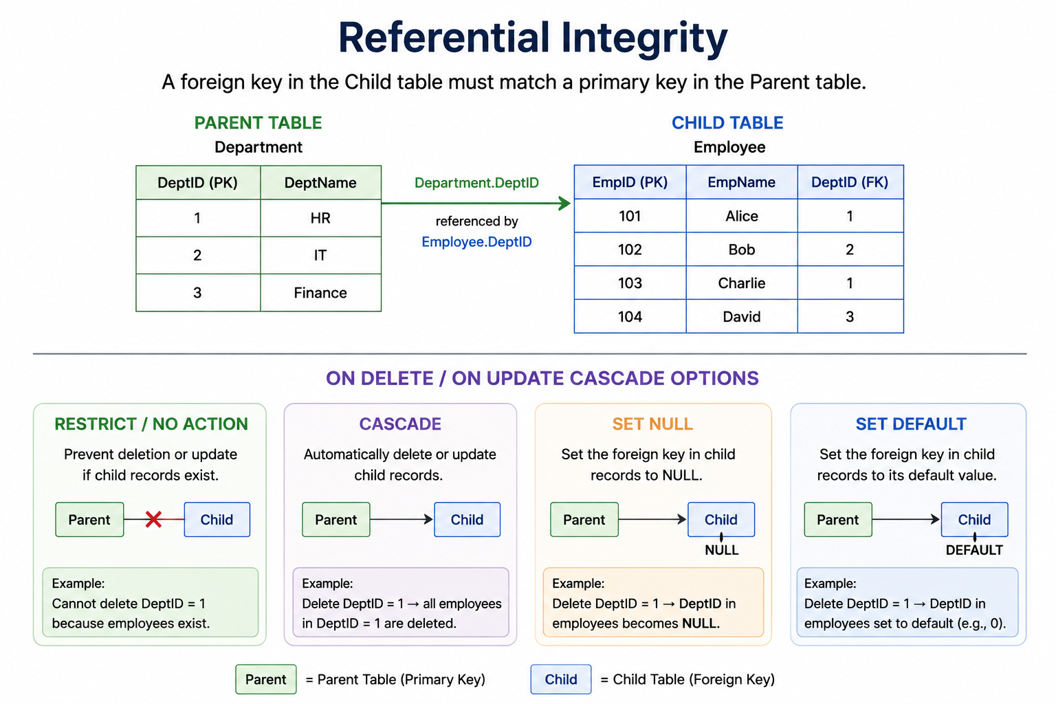
A Foreign Key is an attribute in one table that links to the Primary Key in another table, ensuring referential integrity.
Key Properties:
- Creates a relationship between two tables.
- Value in foreign key column must match a primary key value in the referenced table OR be NULL.
- A table can have multiple foreign keys.
- Prevents orphan records in the database.
Example:
```sql
CREATE TABLE BRANCH (
BRANCH_CODE VARCHAR(10) PRIMARY KEY,
BRANCH_NAME VARCHAR(50)
);
CREATE TABLE STUDENT (
ROLL_NO INT PRIMARY KEY,
NAME VARCHAR(50),
BRANCH_CODE VARCHAR(10),
FOREIGN KEY (BRANCH_CODE) REFERENCES BRANCH(BRANCH_CODE)
);
```
Sample Data:
BRANCH Table:
| BRANCH_CODE | BRANCH_NAME |
|---|---|
| CSE | Computer Science |
| ECE | Electronics |
STUDENT Table:
| ROLL_NO | NAME | BRANCH_CODE |
|---|---|---|
| 101 | Alice | CSE | ← Must exist in BRANCH table
| 102 | Bob | ECE | ← Must exist in BRANCH table
Referential Integrity:
- Cannot insert a STUDENT with BRANCH_CODE that doesn't exist in BRANCH.
- Cannot delete a BRANCH that is referenced by STUDENTs (unless cascading).
Cascading Options:
- ON DELETE CASCADE — deletes related rows.
- ON UPDATE CASCADE — updates related rows.
- SET NULL — sets foreign key to NULL on parent change.
What is denormalization, and how does it differ from normalization?
Denormalization combines tables to improve query performance by adding redundancy — the opposite of normalization.
Denormalization:
- Combines tables to reduce the number of joins needed.
- Adds redundancy intentionally for performance.
- Sacrifices some data integrity for faster read operations.
- Used when read performance is more critical than write performance.
Normalization:
- Reduces redundancy by splitting tables into smaller related tables.
- Enhances data integrity and consistency.
- Optimizes write operations but may slow down complex queries.
Comparison:
| Aspect | Normalization | Denormalization |
|---|---|---|
| Goal | Reduce redundancy | Improve read performance |
| Data Redundancy | Minimized | Increased intentionally |
| Tables | More tables, smaller | Fewer tables, larger |
| Joins | More joins required | Fewer joins needed |
| Read Speed | Slower for complex queries | Faster reads |
| Write Speed | Faster writes | Slower writes (multiple updates) |
| Integrity | High | May have anomalies |
When to Use Denormalization:
- Data warehouses and OLAP systems.
- Reporting databases with heavy reads.
- Systems where query performance is critical.
- When network/disk I/O is a bottleneck.
Example:
- Instead of joining Order and Customer tables every query, store customer_name directly in the Order table — faster reads but customer name updates
require multiple changes.
What is a candidate key in DBMS?
A Candidate Key is a minimal set of attributes that uniquely identifies a tuple in a relation.
Key Properties:
- Uniquely identifies each row in a table.
- Minimal — removing any attribute breaks the uniqueness.
- A table can have multiple candidate keys.
- One candidate key is selected as the Primary Key.
- Other candidate keys become alternate keys.
Example:
```
EMPLOYEE Table:
+--------+----------+--------+--------+
| Emp_ID | Email | SSN | Name |
+--------+----------+--------+--------+
| 1 | a@x.com | 12345 | Alice |
| 2 | b@x.com | 67890 | Bob |
| 3 | c@x.com | 11122 | Carol |
+--------+----------+--------+--------+
```
Candidate Keys:
- Emp_ID — uniquely identifies each employee.
- Email — each email is unique.
- SSN — Social Security Number is unique per person.
Selection:
- Primary Key chosen: Emp_ID (typically a numeric ID).
- Alternate Keys: Email, SSN.
Difference from Other Keys:
Super Key:
- Any superset that uniquely identifies rows (may have extra attributes).
Candidate Key:
- Minimal super key — no redundant attributes.
Primary Key:
- The chosen candidate key for the table.
Alternate Key:
- Candidate keys not chosen as primary.
Why Candidate Keys Matter:
- Help in normalization and database design.
- Identify all possible unique identifiers for entities.
What is the purpose of the SQL SELECT statement?
The SQL SELECT statement retrieves data from one or more tables in a database.
Capabilities:
- Select specific columns to display.
- Apply filters to retrieve specific rows.
- Sort results in ascending or descending order.
- Join multiple tables to combine data.
- Group rows for aggregations.
Basic Syntax:
```sql
SELECT column1, column2, ...
FROM table_name
WHERE condition
ORDER BY column;
```
Common Clauses:
WHERE:
- Filters rows based on conditions.
- Example: `WHERE AGE > 18`
ORDER BY:
- Sorts results (ASC or DESC).
- Example: `ORDER BY NAME ASC`
GROUP BY:
- Groups rows for aggregate functions.
- Example: `GROUP BY DEPARTMENT`
HAVING:
- Filters groups (used with GROUP BY).
- Example: `HAVING COUNT(*) > 5`
Examples:
Simple SELECT:
```sql
SELECT NAME, AGE FROM STUDENT WHERE AGE > 18;
```
SELECT with JOIN:
```sql
SELECT S.NAME, B.BRANCH_NAME
FROM STUDENT S
JOIN BRANCH B ON S.BRANCH_CODE = B.BRANCH_CODE;
```
SELECT with Aggregation:
```sql
SELECT BRANCH, COUNT(*) AS TOTAL
FROM STUDENT
GROUP BY BRANCH;
```
Why SELECT Matters:
- Most frequently used SQL command.
- Foundation for all data analysis and reporting.
- Supports complex queries with subqueries and aggregations.
What is a view in DBMS, and how is it different from a table?
A View is a virtual table created by querying one or more base tables.
Key Characteristics:
- Does not store data physically on its own.
- Dynamically retrieves data when queried.
- Shows data from other tables without storing its own data.
- Defined using a SELECT query.
Creating a View:
```sql
CREATE VIEW Active_Students AS
SELECT Roll_No, Name, Age
FROM Student
WHERE Status = 'Active';
```
Using a View:
```sql
SELECT * FROM Active_Students;
```
View vs Table:
| Aspect | View | Table |
|---|---|---|
| Storage | Doesn't store data | Stores actual data |
| Data Source | Derived from other tables | Self-contained |
| Updates | Reflects base table changes | Independent |
| Performance | Slower (query runs each time) | Faster (direct access) |
| Disk Space | Minimal (only definition stored) | Full data storage |
| Creation | `CREATE VIEW` | `CREATE TABLE` |
Types of Views:
Simple Views:
- Based on a single table, no aggregations.
- Often updatable.
Complex Views:
- Based on multiple tables, may include joins, GROUP BY, aggregates.
- Usually read-only.
Materialized Views:
- Special views that store data physically.
- Refreshed periodically — faster reads.
Benefits of Views:
- Security — hide sensitive columns from users.
- Simplification — abstract complex queries.
- Consistency — provide consistent representation of data.
- Backward compatibility — keep old schema accessible.
What types of relationships exist in DBMS?
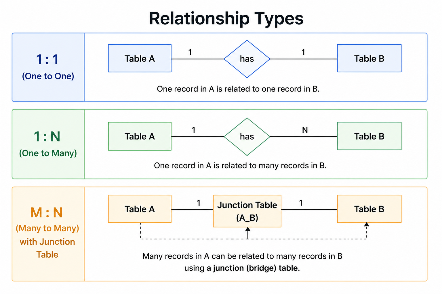
Relationships in DBMS define how data in different tables relate to each other. There are three main types:
One-to-One (1:1):
- Each record in one table relates to exactly one record in another table.
- Used to split a table for security or organization purposes.
- Example: A Person has one Passport — each person has only one passport, and each passport belongs to one person.
```
Person (ID) ←→ Passport (Person_ID)
```
One-to-Many (1:N):
- One record in a table relates to multiple records in another table.
- Most common relationship type.
- Example: A Department has many Employees — one department employs many people, but each employee works in one department.
```
Department (Dept_ID) ←→ Employee (Dept_ID)
1 Many
```
Many-to-Many (M:N):
- Multiple records in one table relate to multiple records in another table.
- Requires a junction (bridge) table to implement.
- Example: Students enroll in Courses — a student takes many courses, and a course has many students.
```
Student → Enrollment ← Course
(junction table connecting both)
```
Junction Table Example:
```sql
CREATE TABLE Enrollment (
Student_ID INT,
Course_ID INT,
PRIMARY KEY (Student_ID, Course_ID),
FOREIGN KEY (Student_ID) REFERENCES Student(ID),
FOREIGN KEY (Course_ID) REFERENCES Course(ID)
);
```
Implementing Relationships:
- One-to-One — foreign key with UNIQUE constraint.
- One-to-Many — foreign key in the "many" side table.
- Many-to-Many — junction table with two foreign keys.
Can you explain the concept of a schema in DBMS?
A schema defines the database structure — acting as a blueprint for data organization.
What a Schema Includes:
- Tables and their columns.
- Views based on tables.
- Relationships between tables.
- Keys (Primary, Foreign, Unique).
- Constraints (NOT NULL, CHECK, etc.).
- Indexes for performance.
- Stored procedures and triggers.
Types of Schemas:
Physical Schema:
- Describes how data is physically stored on disk.
- Includes file organization, block sizes, indexes.
Logical Schema:
- Describes the logical structure — tables, relationships, constraints.
- Most commonly referenced as "the schema".
View Schema (External):
- User-specific views of the database.
- Different users see different subsets.
Three-Level Schema Architecture (ANSI/SPARC):
```
View Level (External) ← User-specific views
↓
Logical Level (Conceptual) ← Tables, columns, relationships
↓
Physical Level (Internal) ← Storage details
```
Schema vs Database Instance:
| Schema | Instance |
|---|---|
| Structure/blueprint | Actual data |
| Rarely changes | Frequently changes |
| Defined at design time | Created at runtime |
Example Schema:
```sql
CREATE SCHEMA university;
CREATE TABLE university.Student (
Roll_No INT PRIMARY KEY,
Name VARCHAR(50) NOT NULL,
Age INT CHECK (Age >= 18)
);
CREATE TABLE university.Course (
Course_ID INT PRIMARY KEY,
Title VARCHAR(100)
);
```
Benefits of Schemas:
- Organize related database objects.
- Security — grant permissions at schema level.
- Namespace — separate objects from different applications.
What are constraints in DBMS?
Constraints are rules enforcing data integrity and validity in a database.
Purpose of Constraints:
- Ensure accurate and consistent data.
- Prevent invalid data entry.
- Enforce business rules at the database level.
- Maintain referential integrity between tables.
Common Types of Constraints:
NOT NULL:
- Column cannot have NULL values.
- Ensures the field always has a value.
PRIMARY KEY:
- Uniquely identifies each row.
- Combination of NOT NULL and UNIQUE.
FOREIGN KEY:
- Links to a primary key in another table.
- Maintains referential integrity.
UNIQUE:
- All values in column must be distinct.
- Allows NULL (unlike primary key).
CHECK:
- Enforces a condition on column values.
- Example: `CHECK (Age >= 18)`.
DEFAULT:
- Provides a default value if none specified.
- Example: `DEFAULT 'Active'`.
Example with Multiple Constraints:
```sql
CREATE TABLE Employee (
Emp_ID INT PRIMARY KEY,
Name VARCHAR(50) NOT NULL,
Email VARCHAR(100) UNIQUE,
Age INT CHECK (Age >= 18),
Status VARCHAR(10) DEFAULT 'Active',
Dept_ID INT,
FOREIGN KEY (Dept_ID) REFERENCES Department(ID)
);
```
Constraint Levels:
Column-level:
- Applied to a single column.
Table-level:
- Applied to multiple columns (composite keys, etc.).
Why Constraints Matter:
- Prevent data corruption.
- Enforce business logic at database level.
- Reduce need for application-level validation.
What are the different categories of constraints in DBMS? Provide examples.
DBMS provides several categories of constraints to enforce data integrity:
NOT NULL:
- Disallows NULL values in a column.
- Ensures the field always has a value.
```sql
Name VARCHAR(50) NOT NULL
```
PRIMARY KEY:
- Uniquely identifies rows without duplicates or NULLs.
- Only one primary key per table.
```sql
ID INT PRIMARY KEY
```
FOREIGN KEY:
- Ensures referential integrity between tables.
- Value must exist in the referenced table.
```sql
BranchCode INT FOREIGN KEY REFERENCES Branch(Code)
```
UNIQUE:
- Enforces distinct values in a column.
- Allows one NULL value (database-dependent).
```sql
Email VARCHAR(100) UNIQUE
```
CHECK:
- Enforces a specific condition on column values.
- Custom validation rules.
```sql
Age INT CHECK (Age >= 18)
```
DEFAULT:
- Assigns a default value if no value provided.
- Reduces explicit value entry.
```sql
Status VARCHAR(10) DEFAULT 'Active'
```
Complete Example:
```sql
CREATE TABLE Employee (
Emp_ID INT PRIMARY KEY,
Name VARCHAR(50) NOT NULL,
Email VARCHAR(100) UNIQUE,
Age INT CHECK (Age >= 18),
Status VARCHAR(10) DEFAULT 'Active',
Dept_ID INT,
FOREIGN KEY (Dept_ID) REFERENCES Department(Dept_ID)
);
```
Adding Constraints Later:
```sql
ALTER TABLE Employee
ADD CONSTRAINT chk_salary CHECK (Salary > 0);
```
Dropping Constraints:
```sql
ALTER TABLE Employee
DROP CONSTRAINT chk_salary;
```
How do DELETE and TRUNCATE commands differ in SQL?
DELETE vs TRUNCATE — Key Differences:
DELETE:
- Removes specific rows based on conditions (WHERE clause).
- Logs each deletion in the transaction log.
- Can be rolled back within a transaction.
- Slower for large tables due to logging.
- DML (Data Manipulation Language) command.
- Triggers DELETE triggers.
```sql
DELETE FROM Student WHERE Age < 18;
DELETE FROM Student; -- removes all rows but logs each
```
TRUNCATE:
- Removes all rows without conditions.
- Does not log individual row deletions.
- Cannot be rolled back (in most databases).
- Much faster than DELETE for large tables.
- DDL (Data Definition Language) command.
- Resets auto-increment counters.
- Does NOT trigger DELETE triggers.
```sql
TRUNCATE TABLE Student;
```
Comparison Table:
| Feature | DELETE | TRUNCATE |
|---|---|---|
| Operation | Row-by-row | Deallocates pages |
| WHERE clause | Yes | No |
| Rollback | Possible | Usually not |
| Transaction Log | Logs each row | Minimal logging |
| Speed | Slower | Faster |
| Triggers | Fires triggers | Doesn't fire triggers |
| Identity reset | No | Yes |
| Type | DML | DDL |
| Locks | Row-level locks | Table-level lock |
When to Use:
Use DELETE when:
- Need to remove specific rows.
- Need to rollback if something goes wrong.
- Need to fire triggers.
Use TRUNCATE when:
- Removing all rows from a large table.
- Performance is critical.
- Don't need to log individual deletions.
Note: DROP is different — it removes the entire table structure, not just data.
What is an index in DBMS, and how does it function?
An index is a data structure that speeds up data retrieval by mapping column values to record locations.
Analogy:
- Similar to a book's table of contents or index — instead of scanning every page, you jump directly to the desired location.
How an Index Works:
1. Index is built on one or more columns of a table.
2. Stores column values and pointers to actual rows.
3. When a query searches by indexed column, DBMS uses the index instead of full table scan.
4. Drastically reduces search time from O(n) to O(log n).
Creating an Index:
```sql
CREATE INDEX idx_name ON Student(Name);
```
Index Data Structures:
B-Tree:
- Most common — balanced tree structure.
- Efficient for range queries and equality searches.
Hash Index:
- Fast for equality lookups.
- Not suitable for range queries.
Bitmap Index:
- Good for columns with few distinct values (e.g., gender, status).
Types of Indexes:
Primary Index:
- Built on primary key automatically.
Secondary Index:
- Built on non-primary key columns.
Clustered Index:
- Physically sorts the table data.
- Only one per table.
Non-Clustered Index:
- Separate structure with pointers.
- Multiple allowed per table.
Benefits:
- Faster SELECT queries with WHERE clauses.
- Improved JOIN performance.
- Speeds up sorting (ORDER BY).
Drawbacks:
- Slows down INSERT, UPDATE, DELETE (index must be updated).
- Uses additional disk space.
When to Use:
- Columns frequently used in WHERE, JOIN, ORDER BY.
- Tables with many rows but selective queries.
What responsibilities does a Database Administrator (DBA) have?
A Database Administrator (DBA) manages and oversees the database environment.
Key Responsibilities:
Database Design:
- Plan and design the database schema.
- Create tables, relationships, and constraints.
- Choose appropriate data types and structures.
Installation and Configuration:
- Install and configure DBMS software.
- Set up servers and clustering.
Backup and Recovery:
- Implement backup strategies (full, incremental, differential).
- Plan disaster recovery procedures.
- Test recovery processes regularly.
Performance Tuning:
- Monitor and optimize query performance.
- Manage indexes for efficient access.
- Tune database parameters and resources.
Security Management:
- Implement user authentication and authorization.
- Manage roles and permissions (GRANT/REVOKE).
- Encrypt sensitive data and audit access.
Data Integrity:
- Enforce constraints and rules.
- Maintain referential integrity across tables.
Upgrades and Patches:
- Apply patches and updates to keep DBMS secure.
- Plan and execute version upgrades.
Troubleshooting:
- Resolve database errors and failures.
- Diagnose performance bottlenecks.
- Manage deadlocks and concurrency issues.
Capacity Planning:
- Monitor storage usage and growth.
- Plan for future scalability needs.
Documentation:
- Maintain documentation of database structure and procedures.
Tools DBAs Use:
- Oracle Enterprise Manager
- SQL Server Management Studio
- pgAdmin (PostgreSQL)
- MySQL Workbench
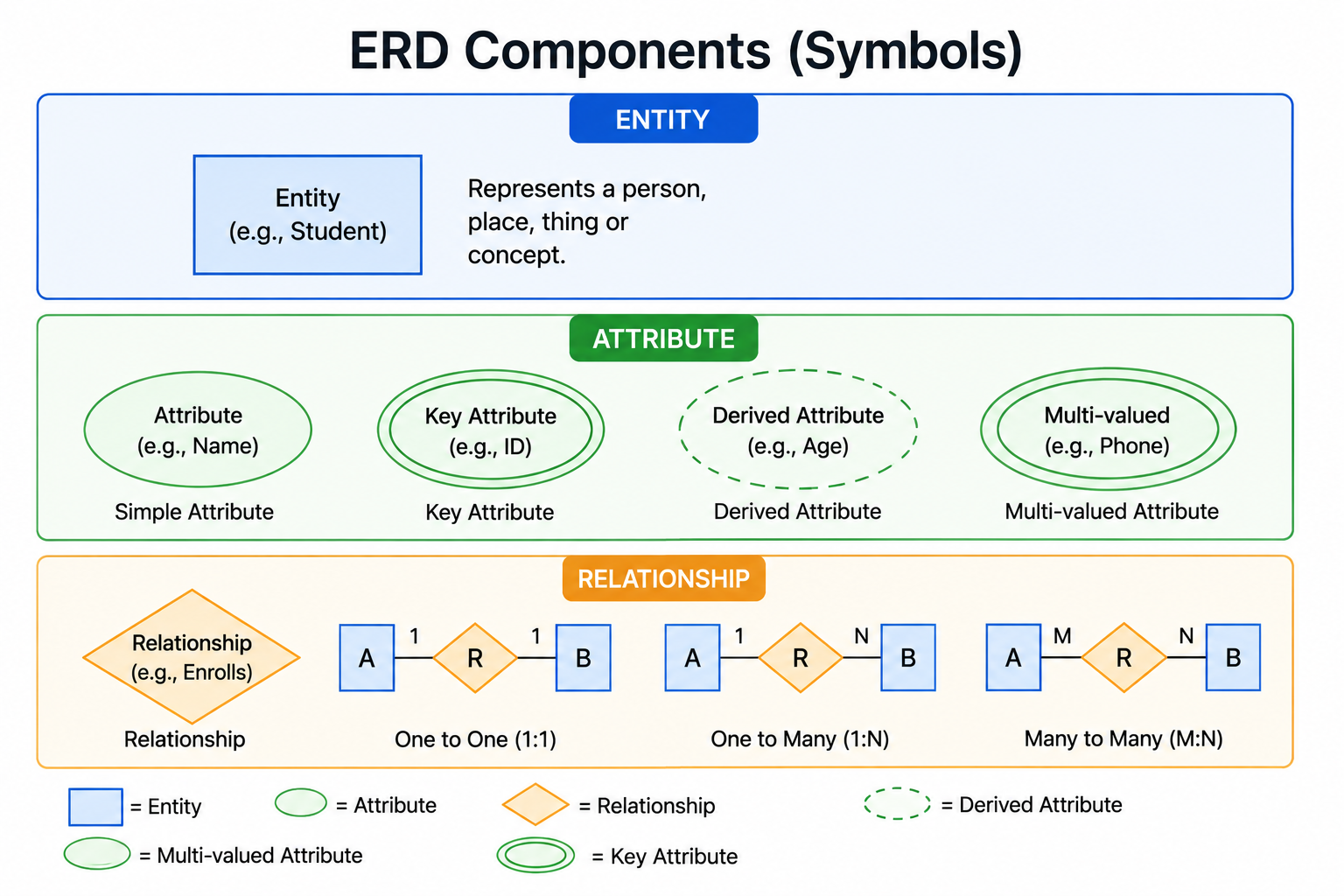
What is an entity-relationship diagram (ERD)?
An Entity-Relationship Diagram (ERD) is a graphical representation of system entities, their attributes, and relationships — used in
database design.
Purpose:
- Visualize database structure before implementation.
- Help in designing efficient database schemas.
- Communicate database design to stakeholders.
Key Components:
Entities:
- Represent real-world objects or concepts.
- Drawn as rectangles.
- Examples: Student, Course, Employee, Department.
Attributes:
- Properties describing an entity.
- Drawn as ovals.
- Examples: Name, Age, Email, ID.
- Types:
- Simple — atomic values (Age, Name).
- Composite — can be divided (Address → Street, City, State).
- Derived — calculated from others (Age from DOB).
- Multivalued — multiple values (Phone Numbers).
Relationships:
- Associations between entities.
- Drawn as diamonds (or lines in modern notations).
- Have cardinality: One-to-One, One-to-Many, Many-to-Many.
Example ERD:
```
[Student] ──< Enrolls >── [Course]
│ │
Name Title
Roll_No Credits
Age Course_ID
```
Cardinality Notations:
- 1:1 — One-to-One
- 1:N — One-to-Many
- M:N — Many-to-Many
ERD Notations:
Chen Notation:
- Original notation with rectangles, ovals, diamonds.
Crow's Foot Notation:
- Modern notation showing cardinality with crow's foot symbols.
UML Notation:
- Uses class-diagram-like representations.
Benefits:
- Clear visualization of database structure.
- Aids in identifying entities and relationships.
- Helps in normalization planning.
- Bridge between business requirements and technical implementation.
Converting ERD to Tables:
- Each entity → table.
- Each attribute → column.
- Relationships → foreign keys or junction tables.
What does a join mean in SQL? Can you name and describe the various types of joins?
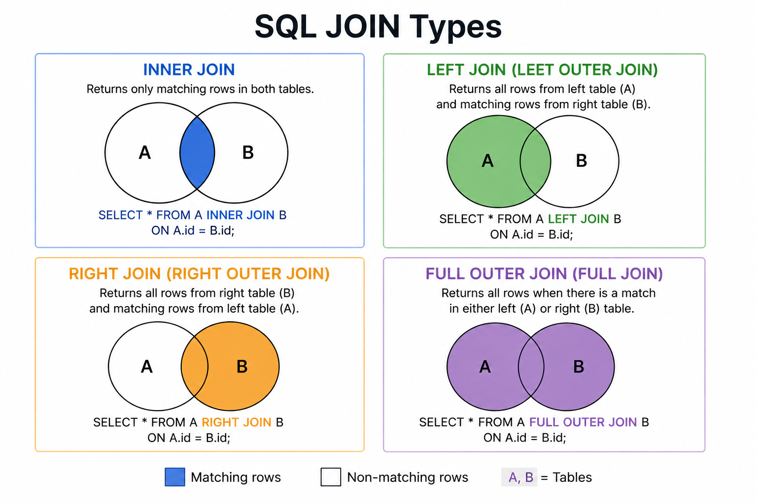
A JOIN in SQL combines columns from multiple tables based on related columns.
Purpose:
- Retrieve related data spread across multiple tables.
- Implement relationships defined by foreign keys.
Types of Joins:
INNER JOIN:
- Returns only matching rows from both tables.
- Most commonly used join.
```sql
SELECT S.Name, C.Title
FROM Student S
INNER JOIN Course C ON S.Course_ID = C.Course_ID;
```
LEFT JOIN (LEFT OUTER JOIN):
- Returns all rows from the left table plus matching rows from the right.
- Non-matching right table rows show as NULL.
```sql
SELECT S.Name, C.Title
FROM Student S
LEFT JOIN Course C ON S.Course_ID = C.Course_ID;
```
RIGHT JOIN (RIGHT OUTER JOIN):
- Returns all rows from the right table plus matching rows from the left.
- Non-matching left table rows show as NULL.
```sql
SELECT S.Name, C.Title
FROM Student S
RIGHT JOIN Course C ON S.Course_ID = C.Course_ID;
```
FULL JOIN (FULL OUTER JOIN):
- Returns all rows from both tables.
- Non-matching rows from either side show as NULL.
```sql
SELECT S.Name, C.Title
FROM Student S
FULL JOIN Course C ON S.Course_ID = C.Course_ID;
```
CROSS JOIN:
- Returns the Cartesian product of both tables.
- Every row from first table combined with every row from second.
```sql
SELECT S.Name, C.Title
FROM Student S
CROSS JOIN Course C;
```
SELF JOIN:
- A table joined with itself.
- Useful for hierarchical data (e.g., Employee-Manager).
```sql
SELECT E1.Name AS Employee, E2.Name AS Manager
FROM Employee E1
JOIN Employee E2 ON E1.Manager_ID = E2.Emp_ID;
```
Visual Representation:
| Join Type | Returns |
|---|---|
| INNER | Intersection only |
| LEFT | All left + matching right |
| RIGHT | All right + matching left |
| FULL | All from both |
| CROSS | Cartesian product |
| SELF | Same table relationships |
What is a subquery in SQL? Could you provide an example?
A subquery is a query within another query — used to provide data for the outer query.
Key Characteristics:
- Enclosed in parentheses.
- Executed first, then result is used by outer query.
- Can appear in SELECT, FROM, WHERE, HAVING clauses.
- Also called nested query or inner query.
Types of Subqueries:
Single-Row Subquery:
- Returns only one value.
- Used with operators like `=`, `<`, `>`, `<=`, `>=`.
Multi-Row Subquery:
- Returns multiple values.
- Used with operators like `IN`, `ANY`, `ALL`.
Multi-Column Subquery:
- Returns multiple columns.
Correlated Subquery:
- References columns from the outer query.
- Executed once for each row of outer query.
Examples:
Single-Row Subquery:
```sql
SELECT Name
FROM Student
WHERE Age > (SELECT AVG(Age) FROM Student);
```
Returns students whose age is greater than the average age.
Multi-Row Subquery with IN:
```sql
SELECT Name
FROM Student
WHERE Course_ID IN (SELECT Course_ID FROM Course WHERE Credits >= 4);
```
Returns students enrolled in courses with 4+ credits.
Correlated Subquery:
```sql
SELECT E1.Name, E1.Salary
FROM Employee E1
WHERE E1.Salary > (
SELECT AVG(E2.Salary)
FROM Employee E2
WHERE E2.Dept_ID = E1.Dept_ID
);
```
Returns employees whose salary is above their department average.
Subquery in FROM:
```sql
SELECT Dept, MaxSalary
FROM (
SELECT Dept, MAX(Salary) AS MaxSalary
FROM Employee
GROUP BY Dept
) AS DeptStats
WHERE MaxSalary > 50000;
```
Subquery vs JOIN:
- Subquery — easier to write for some problems, may be slower.
- JOIN — often more efficient, especially with proper indexes.
- Modern optimizers may convert subqueries to joins internally.
What are aggregate functions in SQL? List some examples.
Aggregate functions operate on groups of rows and return a single value summarizing the group.
Common Aggregate Functions:
COUNT():
- Counts the number of rows.
- `COUNT(*)` counts all rows including NULLs.
- `COUNT(column)` counts non-NULL values in the column.
```sql
SELECT COUNT(*) FROM Student;
SELECT COUNT(Age) FROM Student;
```
SUM():
- Returns the total of numeric values in a column.
- Ignores NULL values.
```sql
SELECT SUM(Salary) FROM Employee;
```
AVG():
- Computes the average of numeric values.
- Ignores NULLs.
```sql
SELECT AVG(Age) FROM Student;
```
MAX():
- Returns the maximum value in a column.
- Works with numbers, strings, and dates.
```sql
SELECT MAX(Salary) FROM Employee;
```
MIN():
- Returns the minimum value in a column.
```sql
SELECT MIN(Age) FROM Student;
```
Other Aggregate Functions:
- STDDEV() — standard deviation.
- VARIANCE() — variance.
- GROUP_CONCAT() / STRING_AGG() — concatenate strings.
Using with GROUP BY:
```sql
SELECT Branch, COUNT(*) AS Students, AVG(Age) AS AvgAge
FROM Student
GROUP BY Branch;
```
Using with HAVING:
```sql
SELECT Branch, COUNT(*) AS Total
FROM Student
GROUP BY Branch
HAVING COUNT(*) > 10;
```
Important Behaviors:
- Aggregate functions ignore NULL values (except COUNT(*)).
- Cannot be used in WHERE clause directly — use HAVING instead.
- Often combined with GROUP BY for grouped statistics.
Example Output:
| Branch | Students | AvgAge |
|---|---|---|
| CSE | 50 | 20.5 |
| ECE | 30 | 21.0 |
| Mechanical | 25 | 20.8 |
How is a transaction defined in DBMS?
A transaction is a set of one or more SQL operations executed as a single unit.
Key Properties:
- Ensures data integrity, consistency, and isolation.
- Either all operations succeed or none do (atomicity).
- Maintains correct state even in case of errors or failures.
Transaction Example — Bank Transfer:
```sql
BEGIN TRANSACTION;
UPDATE Account
SET Balance = Balance - 100
WHERE Account_ID = 1;
UPDATE Account
SET Balance = Balance + 100
WHERE Account_ID = 2;
COMMIT;
```
Why this is a transaction:
- Both updates must succeed together.
- If second update fails, the first must be undone.
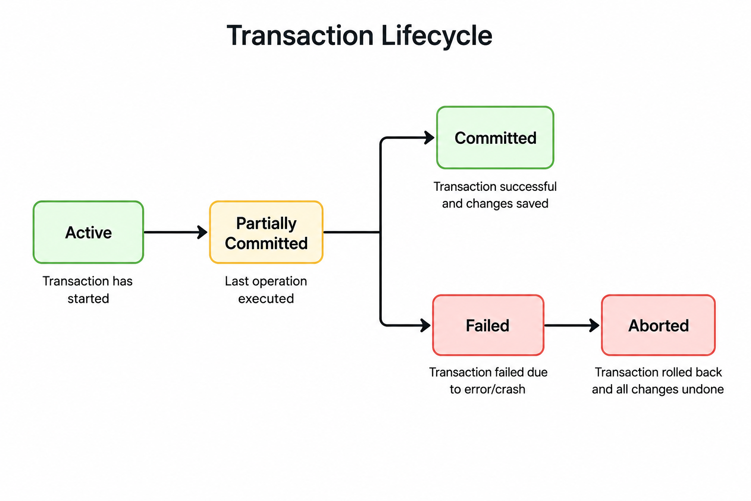
Transaction Lifecycle:
Active State:
- Transaction is being executed.
Partially Committed:
- Last operation has executed, but changes not yet permanent.
Committed:
- All changes are permanently saved to the database.
Failed:
- An error has occurred during execution.
Aborted/Rolled Back:
- All changes are undone, database returns to previous state.
Transaction Control Commands:
BEGIN / START TRANSACTION:
- Marks the start of a transaction.
COMMIT:
- Permanently saves all changes.
ROLLBACK:
- Undoes all changes since the beginning of transaction.
SAVEPOINT:
- Creates a named point to which you can rollback.
Example with SAVEPOINT:
```sql
BEGIN TRANSACTION;
UPDATE Account SET Balance = Balance - 100 WHERE ID = 1;
SAVEPOINT after_debit;
UPDATE Account SET Balance = Balance + 100 WHERE ID = 2;
-- If second update fails:
ROLLBACK TO SAVEPOINT after_debit;
```
Why Transactions Matter:
- Banking systems — money transfers, payments.
- E-commerce — order processing, inventory updates.
- Reservations — hotel bookings, flight tickets.
- Ensure data correctness in concurrent environments.
What does the ACID property signify in DBMS?
ACID properties guarantee reliable transactions in a DBMS.
Atomicity:
- Ensures all operations succeed or none do — all-or-nothing principle.
- Treats the entire transaction as a single unit.
- If any part fails, the entire transaction is rolled back.
Example:
- Bank transfer involves debit from one account and credit to another.
- If credit fails, the debit must be rolled back.
Consistency:
- Maintains a valid database state before and after the transaction.
- All integrity constraints must be satisfied.
- Database moves from one consistent state to another.
Example:
- If total balance must remain constant, the transaction must not violate this.
Isolation:
- Ensures independent transactions — concurrent transactions don't interfere.
- Each transaction appears to execute as if it were the only one running.
- Prevents anomalies like dirty reads, lost updates, and phantom reads.
Isolation Levels:
- Read Uncommitted — lowest isolation.
- Read Committed — common default.
- Repeatable Read — prevents non-repeatable reads.
- Serializable — highest isolation, behaves like serial execution.
Durability:
- Saves committed changes permanently.
- Once a transaction is committed, changes survive system failures.
- Achieved through transaction logs and write-ahead logging (WAL).
Example:
- After bank transfer is committed, even a power failure won't undo it.
Real-World Importance:
| Property | Without It | Example Failure |
|---|---|---|
| Atomicity | Partial updates | Money debited but not credited |
| Consistency | Invalid data | Total balance changes |
| Isolation | Concurrency bugs | Two users overwriting each other |
| Durability | Data loss | Committed transaction lost after crash |
ACID-Compliant Databases:
- PostgreSQL, MySQL (InnoDB), Oracle, SQL Server.
Non-ACID Databases:
- Many NoSQL databases prioritize availability over strict ACID compliance (BASE model).
Can you explain the concept of a stored procedure in DBMS?
A stored procedure is a precompiled set of SQL statements stored in the database.
Key Characteristics:
- Precompiled — improves performance.
- Reusable — can be called multiple times.
- Accepts input parameters.
- Performs operations and returns results.
- Stored on the database server.
Benefits:
- Improved performance — precompiled execution plan.
- Code reusability — write once, use many times.
- Reduced network traffic — execute multiple operations with one call.
- Better security — restrict direct table access, grant only procedure execution.
- Maintainability — change logic in one place.
Creating a Stored Procedure:
```sql
CREATE PROCEDURE GetStudentByAge(@MinAge INT)
AS
BEGIN
SELECT Name, Age, Branch
FROM Student
WHERE Age >= @MinAge;
END;
```
Executing a Stored Procedure:
```sql
EXEC GetStudentByAge @MinAge = 18;
-- or
CALL GetStudentByAge(18); -- MySQL/PostgreSQL syntax
```
Stored Procedure with Multiple Operations:
```sql
CREATE PROCEDURE TransferMoney(
@FromAccount INT,
@ToAccount INT,
@Amount DECIMAL(10,2)
)
AS
BEGIN
BEGIN TRANSACTION;
UPDATE Account
SET Balance = Balance - @Amount
WHERE Account_ID = @FromAccount;
UPDATE Account
SET Balance = Balance + @Amount
WHERE Account_ID = @ToAccount;
COMMIT;
END;
```
Parameter Types:
- IN — input parameter (default).
- OUT — output parameter.
- INOUT — both input and output.
Stored Procedures vs Functions:
| Aspect | Stored Procedure | Function |
|---|---|---|
| Return value | Optional (multiple) | Mandatory (single) |
| Calling | EXEC / CALL | In SELECT statements |
| Side effects | Allowed | Limited |
| Transaction control | Yes | No |
Use Cases:
- Complex business logic that must run on the server.
- Batch processing of records.
- Validation and security layer.
- Common operations like data import, reports.
What are triggers in DBMS? Please give an example.
Triggers are special stored procedures that automatically execute on certain table events.
Key Characteristics:
- Automatically executed — no manual invocation needed.
- Fired on specific events — INSERT, UPDATE, DELETE.
- Used to enforce rules, maintain consistency, or log changes.
- Cannot accept parameters or return values directly.
Types of Triggers:
Based on Timing:
- BEFORE Trigger — executes before the operation.
- AFTER Trigger — executes after the operation.
- INSTEAD OF Trigger — replaces the operation (used with views).
Based on Level:
- Row-Level — fires for each row affected.
- Statement-Level — fires once per SQL statement.
Creating a Trigger:
```sql
CREATE TRIGGER trg_AuditEmployee
AFTER INSERT ON Employee
FOR EACH ROW
BEGIN
INSERT INTO Employee_Audit (Emp_ID, Action, ActionDate)
VALUES (NEW.Emp_ID, 'INSERT', NOW());
END;
```
Real-World Examples:
Audit Logging:
```sql
CREATE TRIGGER trg_LogSalaryChange
AFTER UPDATE OF Salary ON Employee
FOR EACH ROW
BEGIN
INSERT INTO Salary_Log(Emp_ID, OldSalary, NewSalary, ChangeDate)
VALUES (OLD.Emp_ID, OLD.Salary, NEW.Salary, NOW());
END;
```
Enforcing Business Rules:
```sql
CREATE TRIGGER trg_CheckAge
BEFORE INSERT ON Student
FOR EACH ROW
BEGIN
IF NEW.Age < 18 THEN
SIGNAL SQLSTATE '45000'
SET MESSAGE_TEXT = 'Age must be at least 18';
END IF;
END;
```
Maintaining Derived Data:
```sql
CREATE TRIGGER trg_UpdateOrderTotal
AFTER INSERT ON OrderItem
FOR EACH ROW
BEGIN
UPDATE Order
SET Total = Total + NEW.Price * NEW.Quantity
WHERE Order_ID = NEW.Order_ID;
END;
```
Common Use Cases:
- Audit trails — log changes to sensitive data.
- Business rule enforcement — validate complex constraints.
- Cascading actions — update related tables.
- Synchronization — keep redundant data consistent.
Drawbacks of Triggers:
- Hidden logic — can be difficult to debug.
- Performance overhead on every operation.
- Complex dependencies if triggers call other triggers.
- Hard to test and maintain.
How do triggers differ from stored procedures?
Triggers vs Stored Procedures — Key Differences:
Execution:
- Triggers — execute automatically upon specific events; cannot be manually invoked.
- Stored Procedures — must be manually executed using EXEC or CALL.
Invocation:
- Triggers — fired by table events (INSERT, UPDATE, DELETE).
- Stored Procedures — called by users or applications.
Parameters:
- Triggers — cannot accept input parameters.
- Stored Procedures — accept input and return output parameters.
Return Values:
- Triggers — cannot return values to the caller.
- Stored Procedures — can return values via OUT parameters or result sets.
Comparison Table:
| Aspect | Trigger | Stored Procedure |
|---|---|---|
| Execution | Automatic | Manual |
| Trigger event | DML operation | User call |
| Parameters | No | Yes |
| Return values | No | Yes |
| Transaction control | Limited | Full control |
| Use case | Auditing, validation | Business logic |
| Calling other procs | Allowed | Allowed |
| Performance impact | Per row/statement | On demand |
When to Use Triggers:
- Audit logging — automatic recording of changes.
- Enforcing complex business rules that can't be done with constraints.
- Maintaining derived data automatically.
- Sending notifications when data changes.
When to Use Stored Procedures:
- Complex business logic that needs explicit invocation.
- Batch processing of data.
- Encapsulating queries for reuse.
- API-like database operations.
Example Comparison:
Trigger (automatic):
```sql
CREATE TRIGGER trg_audit
AFTER UPDATE ON Employee
FOR EACH ROW
INSERT INTO Audit_Log VALUES (NEW.ID, NOW());
```
Runs automatically after every UPDATE.
Stored Procedure (manual):
```sql
CREATE PROCEDURE UpdateEmployeeSalary(@ID INT, @Salary INT)
AS
UPDATE Employee SET Salary = @Salary WHERE ID = @ID;
```
Must be called: `EXEC UpdateEmployeeSalary @ID=1, @Salary=50000;`
Combination:
- Triggers can call stored procedures for complex logic.
- This combines automation with modularity.
What is the difference between UNION and UNION ALL in SQL?
UNION vs UNION ALL — Key Differences:
UNION:
- Merges query results and removes duplicates.
- Returns distinct values only.
- Slower due to duplicate removal.
- Performs an implicit sort to identify duplicates.
UNION ALL:
- Merges query results but includes duplicates.
- Returns all rows from both queries.
- Faster since no duplicate check is performed.
Syntax:
```sql
SELECT Name FROM Student
UNION
SELECT Name FROM Teacher;
SELECT Name FROM Student
UNION ALL
SELECT Name FROM Teacher;
```
Example:
Student Table:
| Name |
|---|
| Alice |
| Bob |
| Carol |
Teacher Table:
| Name |
|---|
| Bob |
| David |
| Carol |
UNION Result (no duplicates):
| Name |
|---|
| Alice |
| Bob |
| Carol |
| David |
UNION ALL Result (with duplicates):
| Name |
|---|
| Alice |
| Bob |
| Carol |
| Bob |
| David |
| Carol |
Comparison Table:
| Aspect | UNION | UNION ALL |
|---|---|---|
| Duplicates | Removed | Kept |
| Performance | Slower | Faster |
| Sorting | Implicit sort | No sort |
| Memory usage | Higher | Lower |
| Use case | Distinct results | All results |
Rules for UNION and UNION ALL:
- Both queries must have the same number of columns.
- Corresponding columns must have compatible data types.
- Column names in the result come from the first SELECT.
- ORDER BY can only appear in the last SELECT.
When to Use:
Use UNION when:
- You need distinct results.
- Combining queries where duplicates are unwanted.
Use UNION ALL when:
- You want all results including duplicates.
- Performance is critical.
- You're certain there are no duplicates to remove.
- Counting occurrences across multiple sources.
Tip:
- If you know there are no duplicates, always use UNION ALL for better performance.
Can you describe the concept of indexing in DBMS?
Indexing speeds up data retrieval by creating data structures based on column values — like an index in the back of a book.
How Indexing Works:
- Database creates a separate data structure mapping column values to row locations.
- When searching by indexed column, DBMS uses the index instead of scanning every row.
- Reduces search time dramatically — from O(n) to O(log n).
Types of Indexes:
Single-Column Index:
- Built on a single column.
- Most basic and common type.
```sql
CREATE INDEX idx_name ON Student(Name);
```
Composite (Multi-Column) Index:
- Built on multiple columns in sequence.
- Useful for queries filtering by combined criteria.
```sql
CREATE INDEX idx_name_age ON Student(Name, Age);
```
Unique Index:
- Ensures column values are unique.
- Automatically created for PRIMARY KEY and UNIQUE constraints.
```sql
CREATE UNIQUE INDEX idx_email ON Student(Email);
```
Other Index Types:
Clustered Index:
- Physically sorts table data.
- Only one per table.
Non-Clustered Index:
- Separate structure with pointers to data.
- Multiple allowed per table.
Full-Text Index:
- For text search capabilities.
Spatial Index:
- For geographic data.
Bitmap Index:
- For columns with few distinct values.
Index Data Structures:
B-Tree:
- Most common — balanced tree.
- Good for range and equality queries.
Hash Index:
- Fast for exact matches.
- Not suitable for ranges.
Benefits:
- Faster SELECT with WHERE clauses.
- Improved JOIN performance.
- Speeds up ORDER BY and GROUP BY.
Drawbacks:
- Slows down INSERT, UPDATE, DELETE.
- Uses additional disk space.
- Indexes must be maintained during writes.
Best Practices:
- Index frequently queried columns in WHERE clauses.
- Index foreign keys for efficient JOINs.
- Avoid over-indexing — each index has overhead.
- Use composite indexes for multi-column queries.
- Monitor and drop unused indexes.
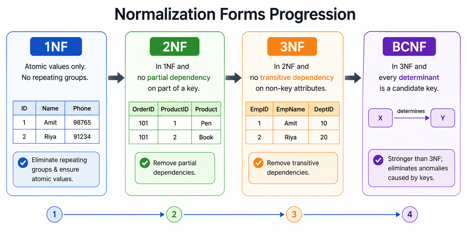
What is normalization in DBMS, and why is it important? Explain the various normal forms (1NF, 2NF, 3NF, BCNF) with examples.
Normalization organizes data to reduce redundancy and maintain integrity by dividing tables and establishing relationships.
Why Normalization Matters:
- Eliminates data redundancy.
- Reduces update, insert, and delete anomalies.
- Improves data integrity.
- Saves storage space.
Normal Forms:
First Normal Form (1NF):
- Each column must contain atomic (indivisible) values.
- No repeating groups or arrays.
- Each row must be unique.
Violation:
| ID | Name | Phones |
|---|---|---|
| 1 | Alice | 123, 456 |
1NF Compliant:
| ID | Name | Phone |
|---|---|---|
| 1 | Alice | 123 |
| 1 | Alice | 456 |
Second Normal Form (2NF):
- Must be in 1NF.
- Removes partial dependencies — non-key attributes must depend on the entire primary key, not just part of it.
- Applies to tables with composite primary keys.
Violation (Student_Course table):
| Student_ID | Course_ID | Student_Name | Course_Name |
|---|---|---|---|
| 1 | C1 | Alice | DBMS |
Here Student_Name depends only on Student_ID (partial dependency).
2NF Compliant — Split into:
- Student(Student_ID, Student_Name)
- Course(Course_ID, Course_Name)
- Enrollment(Student_ID, Course_ID)
Third Normal Form (3NF):
- Must be in 2NF.
- Removes transitive dependencies — non-key attributes should not depend on other non-key attributes.
Violation:
| Emp_ID | Name | Dept_ID | Dept_Name |
|---|---|---|---|
| 1 | Alice | D1 | Engineering |
Dept_Name depends on Dept_ID (transitive dependency).
3NF Compliant — Split into:
- Employee(Emp_ID, Name, Dept_ID)
- Department(Dept_ID, Dept_Name)
Boyce-Codd Normal Form (BCNF):
- A stricter version of 3NF.
- Every determinant must be a candidate key.
- Eliminates anomalies missed by 3NF.
Violation Example:
| Student | Course | Instructor |
|---|---|---|
If each instructor teaches only one course, then Instructor → Course, but Instructor isn't a candidate key.
BCNF Compliant — Split into:
- Student_Instructor(Student, Instructor)
- Instructor_Course(Instructor, Course)
Higher Normal Forms:
- 4NF — eliminates multi-valued dependencies.
- 5NF — eliminates join dependencies.
Trade-offs:
- Higher normalization = better integrity, less redundancy.
- But more joins, potentially slower reads.
- Most production databases stop at 3NF or BCNF.
How do INNER JOIN and OUTER JOIN differ?
INNER JOIN vs OUTER JOIN — Key Differences:
INNER JOIN:
- Returns only matched rows from both tables.
- Excludes rows that don't have matching values.
- Usually faster than OUTER JOIN.
OUTER JOIN:
- Returns matched and unmatched rows.
- Unmatched rows show NULL for missing matches.
- Three types: LEFT, RIGHT, FULL.
Example Tables:
Student Table:
| ID | Name | Course_ID |
|---|---|---|
| 1 | Alice | C1 |
| 2 | Bob | C2 |
| 3 | Carol | NULL |
Course Table:
| Course_ID | Title |
|---|---|
| C1 | DBMS |
| C2 | OS |
| C3 | Networks |
INNER JOIN Result:
```sql
SELECT S.Name, C.Title
FROM Student S
INNER JOIN Course C ON S.Course_ID = C.Course_ID;
```
| Name | Title |
|---|---|
| Alice | DBMS |
| Bob | OS |
Returns only matching rows.
LEFT OUTER JOIN Result:
```sql
SELECT S.Name, C.Title
FROM Student S
LEFT JOIN Course C ON S.Course_ID = C.Course_ID;
```
| Name | Title |
|---|---|
| Alice | DBMS |
| Bob | OS |
| Carol | NULL |
Includes all Students even without matching course.
RIGHT OUTER JOIN Result:
| Name | Title |
|---|---|
| Alice | DBMS |
| Bob | OS |
| NULL | Networks |
Includes all Courses even without matching student.
FULL OUTER JOIN Result:
| Name | Title |
|---|---|
| Alice | DBMS |
| Bob | OS |
| Carol | NULL |
| NULL | Networks |
Includes all rows from both tables.
Comparison Table:
| Aspect | INNER JOIN | OUTER JOIN |
|---|---|---|
| Returns | Only matches | All + matches |
| NULL values | None | For unmatched rows |
| Performance | Faster | Slower |
| Use case | Strict matches | Complete data view |
When to Use:
Use INNER JOIN when:
- You only want rows with matches.
- Performance is critical.
- Unmatched data isn't needed.
Use OUTER JOIN when:
- You need all records from one or both tables.
- Identifying unmatched data (e.g., orphan records).
- Reporting purposes that include all entities.
What is data redundancy in databases, and how can it be minimized?
Data redundancy is the unnecessary repetition of data in a database, causing inconsistency and storage waste.
Problems Caused by Redundancy:
Update Anomalies:
- Same data in multiple places must be updated everywhere.
- Risk of inconsistency if updates miss some occurrences.
Insertion Anomalies:
- Cannot insert certain data without other related data.
Deletion Anomalies:
- Deleting one record may unintentionally remove other important data.
Storage Waste:
- Multiple copies consume more disk space.
Example of Redundancy:
Bad Design (Redundant):
| Order_ID | Customer_Name | Customer_Email | Product |
|---|---|---|---|
| 1 | Alice | alice@x.com | Book |
| 2 | Alice | alice@x.com | Pen |
| 3 | Alice | alice@x.com | Laptop |
Alice's details repeated for every order.
Good Design (Normalized):
Customer Table:
| Cust_ID | Name | Email |
|---|---|---|
| 1 | Alice | alice@x.com |
Order Table:
| Order_ID | Cust_ID | Product |
|---|---|---|
| 1 | 1 | Book |
| 2 | 1 | Pen |
| 3 | 1 | Laptop |
Ways to Minimize Redundancy:
Normalization:
- Apply 1NF, 2NF, 3NF, BCNF to split tables.
- Each piece of data stored only once.
Unique Constraints:
- Use UNIQUE constraints to prevent duplicate entries.
Primary Keys:
- Ensure each record is uniquely identifiable.
Foreign Keys:
- Reference related data instead of duplicating.
Views:
- Create virtual tables to display combined data without duplicating.
Stored Procedures:
- Centralize common operations to avoid logic duplication.
Indexing:
- While not directly reducing redundancy, helps avoid the need to duplicate data for performance.
Trade-offs:
- High normalization → low redundancy but more joins.
- Denormalization → controlled redundancy for read performance.
- Balance based on application needs.
Modern Approach:
- OLTP systems — heavily normalized.
- Data warehouses / OLAP — denormalized for analytics performance.
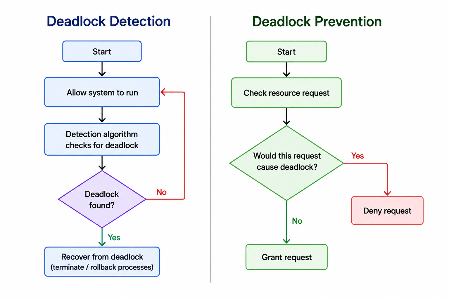
What is a deadlock in DBMS, and what methods can prevent it?
Deadlock occurs when transactions wait indefinitely for each other's resources — none can proceed.
Example of Deadlock:
```
Transaction T1: Locks Row 1, waits for Row 2
Transaction T2: Locks Row 2, waits for Row 1
→ DEADLOCK: Both stuck forever
```
Conditions for Deadlock:
1. Mutual Exclusion — resources not sharable.
2. Hold and Wait — holding resources while waiting for others.
3. No Preemption — resources can't be forcibly taken.
4. Circular Wait — cycle of waiting transactions.
Deadlock Prevention Methods:
Lock Ordering:
- Acquire locks in a consistent global order.
- Prevents circular wait.
- Example: Always lock row with smaller ID first.
Timeouts:
- Set a maximum waiting time for resources.
- Rollback transactions that exceed the timeout.
- Simple but may cause unnecessary rollbacks.
Deadlock Detection:
- Use a wait-for graph to detect cycles.
- If a cycle is detected, rollback one transaction to break it.
- Common in modern DBMS like MySQL, PostgreSQL.
Deadlock Avoidance — Banker's Algorithm:
- Check resource allocation before granting.
- Ensure system stays in a safe state.
Wait-Die Scheme:
- Older transaction waits, younger dies (rolled back) and restarts.
- Based on transaction timestamps.
Wound-Wait Scheme:
- Older transaction wounds (preempts) younger — forces younger to rollback.
- Younger transactions wait for older ones.
Best Practices to Prevent Deadlocks:
Use Short Transactions:
- Keep transactions as short as possible.
- Reduces window for deadlock.
Access Resources in Consistent Order:
- Always access tables and rows in the same order.
Use Lower Isolation Levels:
- Use the lowest isolation level that meets requirements.
- Higher isolation = more locks = more deadlock risk.
Avoid User Interaction During Transactions:
- Don't wait for user input mid-transaction.
Use Optimistic Concurrency Control:
- Check for conflicts at commit time instead of locking.
Recovery from Deadlock:
Victim Selection:
- DBMS chooses a transaction to abort based on:
- Transaction age.
- Resources held.
- Progress made.
Rollback:
- Aborted transaction is rolled back.
- Other transactions can proceed.
Restart:
- Aborted transaction is automatically restarted by application.
What is a database cursor, and how is it utilized?
A cursor is a pointer to a query result set, allowing row-by-row processing.
Purpose:
- Process query results one row at a time.
- Useful when set-based operations aren't sufficient.
- Provides programmatic control over result navigation.
Types of Cursors:
Implicit Cursors:
- Automatically created by the DBMS for SQL statements.
- Used internally for INSERT, UPDATE, DELETE, SELECT INTO.
- Programmer doesn't manage them directly.
Explicit Cursors:
- Programmer-defined for complex query processing.
- Provide explicit control over fetching rows.
- Used in stored procedures and functions.
Cursor Lifecycle:
1. Declare:
- Define the cursor with a SELECT statement.
2. Open:
- Execute the query and prepare for fetching.
3. Fetch:
- Retrieve rows one by one.
4. Close:
- Release the cursor resources.
Example — Oracle PL/SQL:
```sql
DECLARE
CURSOR student_cursor IS
SELECT Name, Age FROM Student WHERE Age > 18;
v_name Student.Name%TYPE;
v_age Student.Age%TYPE;
BEGIN
OPEN student_cursor;
LOOP
FETCH student_cursor INTO v_name, v_age;
EXIT WHEN student_cursor%NOTFOUND;
DBMS_OUTPUT.PUT_LINE(v_name || ' - ' || v_age);
END LOOP;
CLOSE student_cursor;
END;
```
Example — SQL Server T-SQL:
```sql
DECLARE @Name VARCHAR(50), @Age INT;
DECLARE student_cursor CURSOR FOR
SELECT Name, Age FROM Student;
OPEN student_cursor;
FETCH NEXT FROM student_cursor INTO @Name, @Age;
WHILE @@FETCH_STATUS = 0
BEGIN
PRINT @Name + ' - ' + CAST(@Age AS VARCHAR);
FETCH NEXT FROM student_cursor INTO @Name, @Age;
END;
CLOSE student_cursor;
DEALLOCATE student_cursor;
```
Cursor Properties:
Scrollable:
- Can move forward and backward through results.
Forward-Only:
- Can move only forward (default, faster).
Updatable:
- Can modify rows while iterating.
Read-Only:
- Cannot modify rows.
When to Use Cursors:
- Complex row-by-row processing that can't be done with set operations.
- Reporting with custom formatting for each row.
- Procedural logic that depends on each row's values.
Drawbacks:
- Slower than set-based operations.
- More memory usage.
- Can cause locking issues.
Best Practice:
- Avoid cursors when set-based SQL operations can do the job.
- Use cursors only when absolutely necessary.
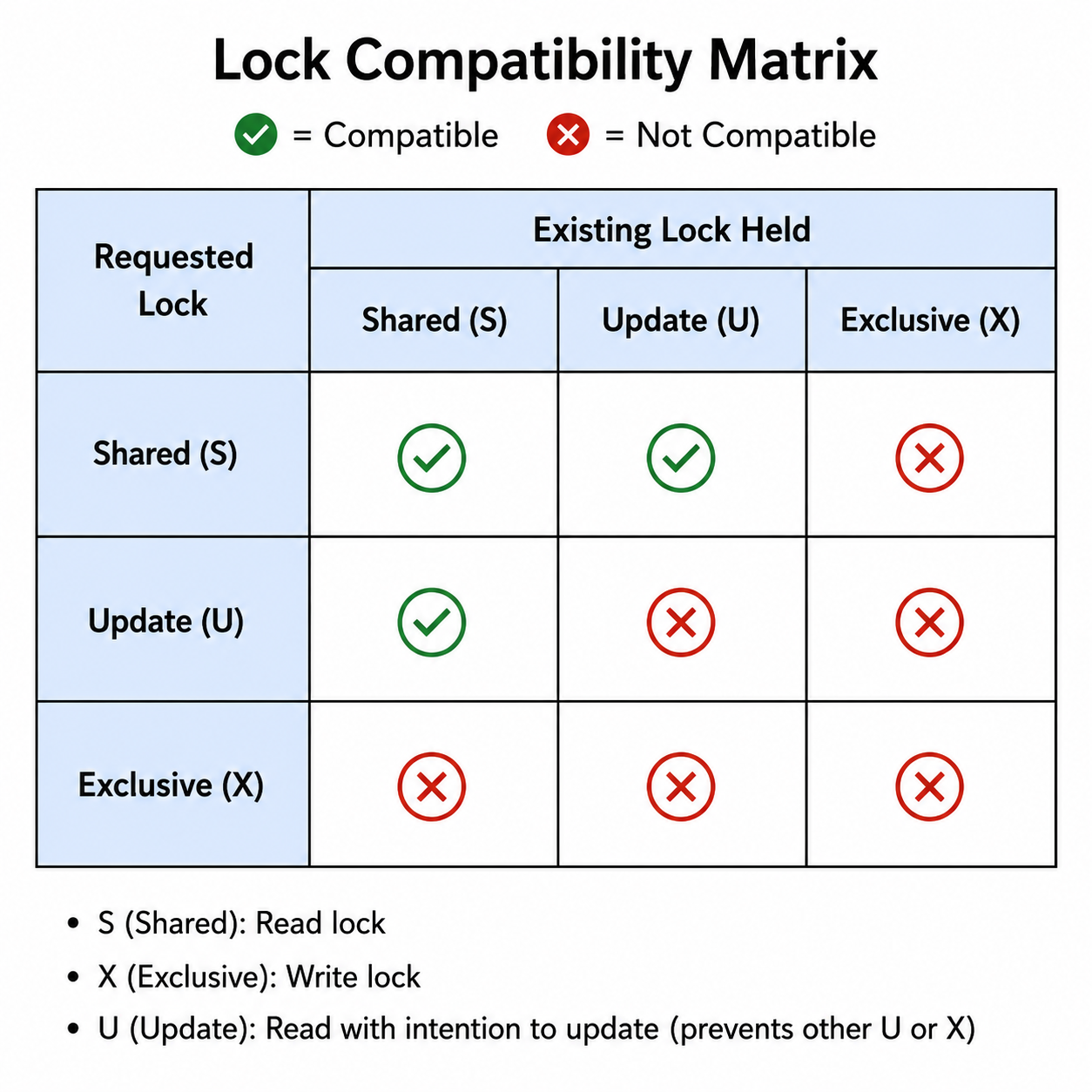
What are the different types of locks used in databases?
Databases use various lock types to ensure concurrency control and prevent conflicts.
Common Lock Types:
Shared Lock (S Lock):
- Allows multiple transactions to read the same data simultaneously.
- Blocks any transaction from writing.
- Also called Read Lock.
```sql
SELECT * FROM Student WHERE ID = 1 FOR SHARE;
```
Exclusive Lock (X Lock):
- Prevents other transactions from reading or writing the data.
- Acquired for UPDATE and DELETE operations.
- Also called Write Lock.
```sql
SELECT * FROM Student WHERE ID = 1 FOR UPDATE;
```
Intent Lock:
- Signals an intention to acquire a more specific lock.
- Helps the lock manager detect conflicts quickly.
- Types:
- Intent Shared (IS) — intention to acquire shared locks.
- Intent Exclusive (IX) — intention to acquire exclusive locks.
Update Lock (U Lock):
- Used before acquiring an exclusive lock.
- Prevents deadlocks when multiple transactions want to update the same data.
- Only one transaction can hold an update lock at a time.
Lock Compatibility Matrix:
| | Shared | Exclusive | Update |
|---|---|---|---|
| Shared | ✓ | ✗ | ✓ |
| Exclusive | ✗ | ✗ | ✗ |
| Update | ✓ | ✗ | ✗ |
Lock Granularity:
Database-Level Lock:
- Locks the entire database.
- Rarely used due to performance impact.
Table-Level Lock:
- Locks an entire table.
- Used for bulk operations.
Page-Level Lock:
- Locks a disk page.
Row-Level Lock:
- Locks individual rows.
- Most granular and concurrent.
Column-Level Lock:
- Locks specific columns (rare).
Lock Modes:
Pessimistic Locking:
- Assumes conflicts will happen — locks data before reading.
- Used in high-contention systems.
Optimistic Locking:
- Assumes conflicts are rare — checks at commit time.
- Uses version numbers or timestamps.
Two-Phase Locking (2PL):
- Growing Phase — acquire locks.
- Shrinking Phase — release locks.
- Ensures serializability.
Deadlock Risk:
- Locks can lead to deadlocks if transactions wait for each other.
- DBMS uses timeout or detection algorithms to resolve.
Best Practices:
- Use lowest level of locking that meets requirements.
- Keep transactions short to release locks quickly.
- Access resources in consistent order.
- Choose appropriate isolation level.
How does a clustered index differ from a non-clustered index?
Clustered vs Non-Clustered Index — Key Differences:
Clustered Index:
- Physically sorts data rows in the table based on the indexed column.
- Only one clustered index can exist per table (since data can be sorted in only one order).
- Data and index are stored together.
- Typically created on the primary key by default.
Non-Clustered Index:
- Stores a separate structure with pointers to the actual data rows.
- Multiple non-clustered indexes can exist per table.
- Data is not physically sorted by this index.
Visual Representation:
Clustered Index:
```
Index → Data (sorted by index column)
[Leaf nodes contain actual data]
```
Non-Clustered Index:
```
Index → Pointers → Data
[Leaf nodes contain row pointers]
```
Example:
Clustered Index on Employee_ID:
| Emp_ID | Name | Salary |
|---|---|---|
| 1 | Alice | 50000 |
| 2 | Bob | 60000 |
| 3 | Carol | 55000 |
Rows physically sorted by Emp_ID.
Non-Clustered Index on Name:
```
Index Structure:
Alice → Pointer to Row with Emp_ID=1
Bob → Pointer to Row with Emp_ID=2
Carol → Pointer to Row with Emp_ID=3
```
Pointers point to actual data, which isn't sorted by Name.
Comparison Table:
| Aspect | Clustered Index | Non-Clustered Index |
|---|---|---|
| Storage | Data sorted physically | Separate index structure |
| Number per table | One | Multiple (typically 999+) |
| Speed (for indexed col) | Faster | Slower (extra lookup) |
| Disk space | Minimal extra | Additional space |
| Insert/Update speed | Slower (re-sort) | Faster |
| Best for | Range queries, ORDER BY | Specific lookups |
| Default | On PRIMARY KEY | Manually created |
When to Use:
Clustered Index:
- Primary key (default).
- Columns used in range queries (BETWEEN, ORDER BY).
- Columns with high uniqueness.
- Columns frequently used in JOINs.
Non-Clustered Index:
- Frequently queried columns in WHERE clauses.
- Foreign keys for efficient JOINs.
- Columns used in GROUP BY.
- When you need multiple indexes.
Performance Considerations:
Clustered Index Pros:
- Faster retrieval of indexed column.
- Efficient range queries.
Clustered Index Cons:
- Slower INSERT/UPDATE as rows may need rearranging.
- Choosing the wrong column can hurt performance.
Non-Clustered Index Pros:
- Multiple can coexist.
- Doesn't affect physical ordering.
Non-Clustered Index Cons:
- Extra lookup step — slower than clustered.
- More disk space required.
Tip:
- Use clustered index on columns frequently used in range queries.
- Use non-clustered indexes on columns used for lookups.
Why are the COMMIT and ROLLBACK operations important?
COMMIT and ROLLBACK are essential for maintaining atomicity and durability of transactions.
COMMIT:
- Permanently saves all transaction changes to the database.
- Once committed, changes cannot be undone through ROLLBACK.
- Ends the current transaction successfully.
- Releases all locks held by the transaction.
ROLLBACK:
- Undoes all changes made by the current transaction.
- Restores the database to its previous state before the transaction began.
- Used when an error occurs or operation should be cancelled.
- Releases all locks held by the transaction.
Why They're Important:
Ensure Atomicity:
- COMMIT confirms all operations succeed together.
- ROLLBACK ensures all-or-nothing behavior on failure.
Maintain Durability:
- After COMMIT, changes survive system failures.
- Even if the database crashes, committed data is preserved.
Provide Error Recovery:
- ROLLBACK undoes changes when errors occur.
- Database state remains consistent despite failures.
Enable Safe Operations:
- Test operations before making them permanent.
- Cancel operations that produce undesired results.
Example — Bank Transfer:
```sql
BEGIN TRANSACTION;
UPDATE Account
SET Balance = Balance - 1000
WHERE Account_ID = 1;
UPDATE Account
SET Balance = Balance + 1000
WHERE Account_ID = 2;
-- Check if both updates succeeded
IF @@ERROR = 0
COMMIT;
ELSE
ROLLBACK;
```
Example with Error Handling:
```sql
BEGIN TRY
BEGIN TRANSACTION;
INSERT INTO Orders (Customer_ID, Total) VALUES (1, 500);
UPDATE Inventory SET Stock = Stock - 1 WHERE Product_ID = 100;
COMMIT;
END TRY
BEGIN CATCH
ROLLBACK;
PRINT 'Error occurred: ' + ERROR_MESSAGE();
END CATCH;
```
SAVEPOINT — Partial Rollback:
```sql
BEGIN TRANSACTION;
INSERT INTO Orders VALUES (1, 500);
SAVEPOINT after_order;
UPDATE Inventory SET Stock = Stock - 1;
-- If inventory update fails:
ROLLBACK TO SAVEPOINT after_order;
COMMIT; -- Order saved, inventory rolled back
```
COMMIT vs ROLLBACK:
| Aspect | COMMIT | ROLLBACK |
|---|---|---|
| Effect | Saves changes | Undoes changes |
| Permanence | Permanent | Restores previous state |
| When used | Success scenarios | Error scenarios |
| Locks | Released | Released |
| Data | Visible to all transactions | Hidden, never visible |
Auto-Commit Mode:
- Most databases support auto-commit — each statement is automatically committed.
- For multi-statement transactions, disable auto-commit and use explicit COMMIT/ROLLBACK.
Real-World Importance:
Banking Systems:
- Ensure money transfers are atomic.
E-commerce:
- Prevent partial order processing.
Inventory Management:
- Maintain consistent stock levels.
Reservations:
- Prevent double-booking.
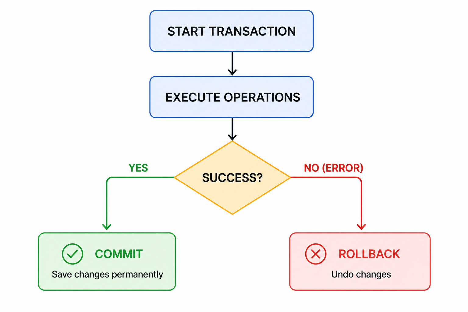
What is the difference between a superkey and a candidate key?
Superkey vs Candidate Key — Key Differences:
Superkey:
- Any set of attributes that uniquely identifies rows in a table.
- May contain extra (redundant) attributes beyond what's needed.
- Every table has at least one superkey (all attributes combined).
Candidate Key:
- A minimal superkey — no redundant attributes.
- Removing any attribute breaks uniqueness.
- Multiple candidate keys can exist; one is chosen as Primary Key.
Example:
Employee Table:
| Emp_ID | Email | SSN | Name | Age |
|---|---|---|---|---|
| 1 | alice@x.com | 12345 | Alice | 25 |
| 2 | bob@x.com | 67890 | Bob | 30 |
Superkeys (uniquely identify rows):
- {Emp_ID}
- {Email}
- {SSN}
- {Emp_ID, Name}
- {Emp_ID, Email, SSN}
- {Email, Age}
- {Emp_ID, Email, SSN, Name, Age} — all attributes
Candidate Keys (minimal superkeys):
- {Emp_ID}
- {Email}
- {SSN}
These cannot have attributes removed without losing uniqueness.
Why {Emp_ID, Name} is NOT a Candidate Key:
- Name is redundant — Emp_ID alone uniquely identifies rows.
- A candidate key must be minimal.
Comparison Table:
| Aspect | Superkey | Candidate Key |
|---|---|---|
| Definition | Any set uniquely identifying rows | Minimal set uniquely identifying rows |
| Redundancy | May have extras | No redundant attributes |
| Number | Many possible | Fewer (subset of superkeys) |
| Relationship | Superset | Subset of superkeys |
Key Hierarchy:
```
Superkey (broadest)
↓
Candidate Key (minimal superkeys)
↓
Primary Key (chosen candidate key)
↓
Alternate Keys (other candidate keys)
```
Mathematical Relationship:
- Every candidate key is a superkey.
- Not every superkey is a candidate key.
- The primary key is the candidate key chosen for the table.
Why Both Concepts Matter:
Superkey:
- Useful for understanding all possible unique identifiers.
- Helps in initial database analysis.
Candidate Key:
- Used in normalization to identify potential primary keys.
- Helps choose the best identifier for the table.
Selecting Primary Key from Candidates:
- Choose the simplest (fewest attributes).
- Prefer stable values (won't change).
- Often numeric IDs over strings.
- Smaller storage size = better index performance.
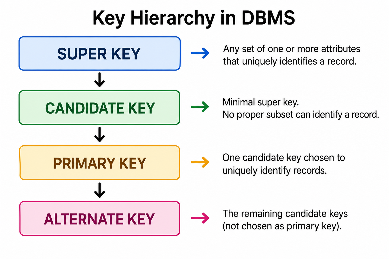
How do primary keys differ from unique keys?
Primary Key vs Unique Key — Key Differences:
Primary Key:
- Uniquely identifies records in a table.
- Disallows NULL values.
- Only one primary key per table.
- Can be a composite key (multiple columns).
- Automatically creates a clustered index (in most databases).
Unique Key:
- Ensures uniqueness in a column or combination.
- Allows NULL values (typically one NULL per column).
- Multiple unique keys permitted per table.
- Automatically creates a non-clustered index (in most databases).
Example:
```sql
CREATE TABLE Employee (
Emp_ID INT PRIMARY KEY, -- Primary Key
Email VARCHAR(100) UNIQUE, -- Unique Key
SSN VARCHAR(20) UNIQUE, -- Another Unique Key
Phone VARCHAR(15) UNIQUE, -- Another Unique Key
Name VARCHAR(50) NOT NULL
);
```
Comparison Table:
| Aspect | Primary Key | Unique Key |
|---|---|---|
| NULL values | Not allowed | Allowed (typically one) |
| Number per table | One | Multiple |
| Index type | Clustered (default) | Non-clustered (default) |
| Purpose | Identify records | Ensure uniqueness |
| Foreign Key reference | Yes | Yes |
| Automatic naming | PK_TableName | UQ_TableName |
Behavior Examples:
Primary Key:
```sql
INSERT INTO Employee (Emp_ID, Email, Name)
VALUES (1, 'alice@x.com', 'Alice');
INSERT INTO Employee (Emp_ID, Email, Name)
VALUES (NULL, 'bob@x.com', 'Bob');
-- ERROR: Primary Key cannot be NULL
INSERT INTO Employee (Emp_ID, Email, Name)
VALUES (1, 'carol@x.com', 'Carol');
-- ERROR: Duplicate Primary Key
```
Unique Key:
```sql
INSERT INTO Employee (Emp_ID, Email, Name)
VALUES (1, NULL, 'Alice');
-- OK: Unique Key allows NULL
INSERT INTO Employee (Emp_ID, Email, Name)
VALUES (2, NULL, 'Bob');
-- May FAIL: Some DBMS allow only one NULL
INSERT INTO Employee (Emp_ID, Email, Name)
VALUES (3, 'alice@x.com', 'Carol');
-- ERROR: Duplicate Email
```
Use Cases:
Primary Key:
- The main identifier for a table.
- Used for foreign key references.
- Should be stable and unique.
- Often a synthetic ID (auto-increment).
Unique Key:
- Enforce business rules on uniqueness.
- Examples: email addresses, phone numbers, SSN, license plates.
- Allow optional fields that must be unique when provided.
Multiple Approach:
```sql
CREATE TABLE User (
User_ID INT PRIMARY KEY, -- System identifier
Email VARCHAR(100) UNIQUE NOT NULL, -- Business identifier
Username VARCHAR(50) UNIQUE NOT NULL,
Phone VARCHAR(15) UNIQUE -- Optional unique
);
```
Tips:
- Use PRIMARY KEY for the main row identifier.
- Use UNIQUE for additional uniqueness constraints.
- Both improve query performance through automatic indexing.
What is referential integrity in DBMS?
Referential Integrity ensures foreign keys correspond to primary or unique keys in related tables, maintaining **consistent
relationships and preventing orphan records**.
Core Rule:
- Foreign key values must either:
- Match a primary/unique key value in the referenced table, OR
- Be NULL (if allowed).
Purpose:
- Prevent invalid references between tables.
- Maintain logical consistency of data.
- Avoid orphan records (records pointing to non-existent parents).
Example:
Department Table (Parent):
| Dept_ID | Dept_Name |
|---|---|
| 1 | Engineering |
| 2 | HR |
| 3 | Finance |
Employee Table (Child):
| Emp_ID | Name | Dept_ID |
|---|---|---|
| 101 | Alice | 1 | ← Valid: Dept 1 exists
| 102 | Bob | 2 | ← Valid: Dept 2 exists
| 103 | Carol | 5 | ← INVALID: Dept 5 doesn't exist!
Creating the Foreign Key:
```sql
CREATE TABLE Employee (
Emp_ID INT PRIMARY KEY,
Name VARCHAR(50),
Dept_ID INT,
FOREIGN KEY (Dept_ID) REFERENCES Department(Dept_ID)
);
```
Referential Integrity Rules Enforced:
INSERT:
- Cannot insert an Employee with a Dept_ID that doesn't exist in Department.
UPDATE:
- Cannot update Employee's Dept_ID to a value not in Department.
DELETE:
- Cannot delete a Department that is referenced by any Employee (default behavior).
Cascading Actions:
ON DELETE CASCADE:
- Deleting a parent automatically deletes related child records.
```sql
FOREIGN KEY (Dept_ID) REFERENCES Department(Dept_ID)
ON DELETE CASCADE;
```
ON UPDATE CASCADE:
- Updating a parent's primary key automatically updates related child records.
```sql
FOREIGN KEY (Dept_ID) REFERENCES Department(Dept_ID)
ON UPDATE CASCADE;
```
ON DELETE SET NULL:
- Sets child's foreign key to NULL when parent is deleted.
```sql
FOREIGN KEY (Dept_ID) REFERENCES Department(Dept_ID)
ON DELETE SET NULL;
```
ON DELETE SET DEFAULT:
- Sets child's foreign key to a default value.
ON DELETE RESTRICT (default):
- Prevents deletion of parent if children exist.
Why Referential Integrity Matters:
Data Consistency:
- Prevents inconsistent data across related tables.
Preventing Orphan Records:
- Ensures every foreign key has a valid reference.
Business Logic Enforcement:
- Relationships defined in design are enforced at the database level.
Reduces Application-Level Validation:
- Database handles validation, reducing code complexity.
Example of Violation Prevention:
```sql
-- This will FAIL:
INSERT INTO Employee (Emp_ID, Name, Dept_ID)
VALUES (104, 'Dave', 99);
-- ERROR: Dept_ID 99 doesn't exist in Department
-- This will FAIL:
DELETE FROM Department WHERE Dept_ID = 1;
-- ERROR: Employees still reference Dept_ID 1
```
Best Practices:
- Always define foreign key constraints for related tables.
- Choose appropriate cascading actions based on business needs.
- Use NOT NULL on foreign keys when the relationship is mandatory.
- Consider performance impact of cascading actions in large tables.