Machine Learning Interview Questions

• Images marked with ★ are AI-generated.

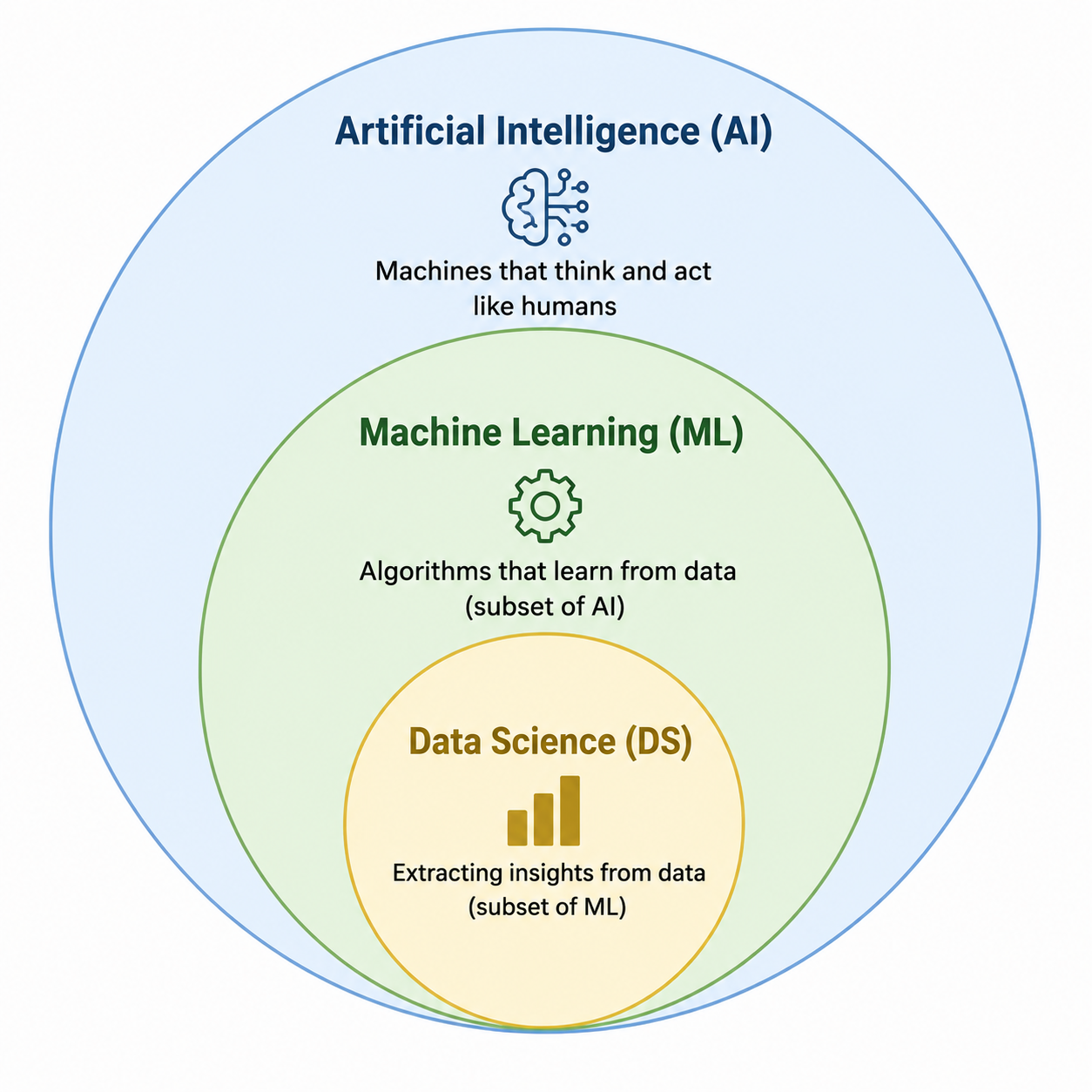
How would you define Machine Learning (ML), and in what ways does it differ from Artificial Intelligence (AI) and Data Science?

GoogleAmazonMicrosoftMetaApple

Solution

Machine Learning (ML) is a branch of Artificial Intelligence that focuses on creating algorithms that can learn from data. Instead of using fixed programming rules, these algorithms identify patterns in data and use them to make predictions or decisions that improve over time.

AI (Artificial Intelligence):

•A broad field aimed at building systems that imitate human intelligence.

•Examples: Chatbots, autonomous vehicles.

ML (Machine Learning):

•A subset of AI that learns from data patterns to predict or decide.

•Examples: Spam filters, recommendation systems.

Data Science:

•A domain focused on extracting insights and knowledge from data.

•Examples: Analyzing sales trends, segmenting customers.

Key Distinction:

•AI is the broadest concept.

•ML is a way to achieve AI.

•Data Science uses ML and statistics to extract insights from data.

How would you define Machine Learning (ML), and in what ways does it differ from Artificial Intelligence (AI) and Data Science? image 1

Figure 1: ★ Machine Learning vs Artificial Intelligence vs Data Science

What does overfitting mean in the context of machine learning, and what strategies can be used to prevent it?

GoogleAmazonMicrosoftMetaNetflix

Solution

Overfitting happens when a model learns both the true patterns and noise from training data, leading to excellent training accuracy but poor performance on new data.

Ways to Prevent Overfitting:

Early Stopping:

•Halt training when validation accuracy no longer improves.

Regularization:

•Use L1 (Lasso) or L2 (Ridge) methods to penalize large weights.

Cross-Validation:

•Apply k-fold cross-validation to check generalization.

Dropout (Neural Networks):

•Randomly omit neurons during training to prevent over-reliance.

Simpler Models:

•Choose less complex models when feasible.

Underfitting occurs when a model is too simple to capture patterns.

To fix underfitting:

•Use more complex models.

•Add relevant features.

•Reduce regularization.

•Train for longer.

Can you explain what Regularization is in machine learning?

GoogleAmazonMicrosoftMetaNetflix

Solution

Regularization reduces model complexity and prevents overfitting by adding a penalty to the loss function that discourages large feature weights.

Regularization Methods:

L1 Regularization (Lasso):

•Adds the sum of absolute weight values as a penalty.

•Can shrink some weights to zero, performing automatic feature selection.

•Best when many features are irrelevant.

L2 Regularization (Ridge):

•Adds the sum of squared weights as a penalty.

•Reduces large coefficients but does not eliminate them.

•Best when all features matter but overfitting is a concern.

Elastic Net:

•Combines both L1 and L2 penalties for balanced feature selection and weight reduction.

Dropout (Neural Networks):

•Randomly drops nodes during training to avoid over-reliance on specific neurons.

Why Regularization Matters:

•Without regularization, models memorize training data and fail to generalize.

•Adding a penalty forces the model to find simpler, more generalizable patterns.

Can you explain what Regularization is in machine learning? image 1

Figure 3: ★ Regularization in Machine Learning

What are Lasso and Ridge Regularization, and how do they contribute to Elastic Net Regularization?

GoogleAmazonMicrosoftMetaNetflix

Solution

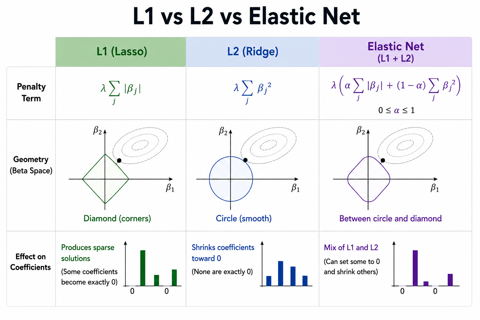
Lasso Regularization (L1):

•Adds the sum of absolute weights as a penalty to the loss function.

•Can shrink weights to zero, effectively performing feature selection.

Loss = MSE + λ × Σ|wᵢ|

Ridge Regularization (L2):

•Adds the sum of squared weights as a penalty.

•Reduces large weights but keeps all features (no zero weights).

Loss = MSE + λ × Σwᵢ²

Key Differences:

Lasso (L1):

•Can zero out weights → good for feature selection.

•Ideal when many features are irrelevant.

Ridge (L2):

•Reduces weights but keeps all features.

•Use when all features matter but overfitting is a concern.

Elastic Net:

•Blends both L1 and L2 penalties together.

•Balances feature selection (L1) and weight shrinkage (L2).

•Especially useful when features are correlated.

Loss = MSE + λ₁ × Σ|wᵢ| + λ₂ × Σwᵢ²

What are the various techniques used to evaluate machine learning models?

GoogleAmazonMicrosoftMetaApple

Solution

Train-Test Split:

•Divide data into training and testing sets (e.g., 70:30 or 80:20) to assess model performance on new data.

Cross-Validation:

•Split data into k folds, train on k-1, validate on the remaining fold, then average results.

Confusion Matrix (Classification):

•Counts True Positives (TP), True Negatives (TN), False Positives (FP), and False Negatives (FN).

Accuracy:

•Ratio of correct predictions to total predictions.

Accuracy = (TP + TN) / (TP + TN + FP + FN)

Precision:

•Correct positive predictions divided by all predicted positives.

Precision = TP / (TP + FP)

Recall (Sensitivity):

•Correct positive predictions divided by total actual positives.

Recall = TP / (TP + FN)

F1-Score:

•Harmonic mean of Precision and Recall.

F1 = 2 × (Precision × Recall) / (Precision + Recall)

ROC Curve and AUC:

•Measures the model's ability to distinguish between classes.

Loss Functions (Regression/Classification):

•MAE, MSE, RMSE for regression; Cross-Entropy for classification.

Could you describe what a Confusion Matrix is?

AmazonGoogleMicrosoftMetaApple

Solution

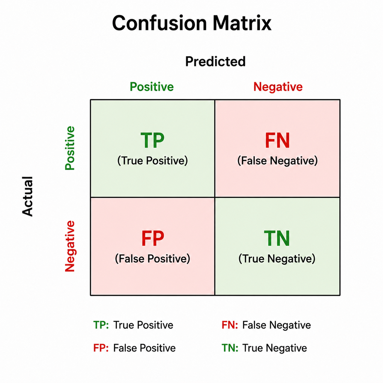
A Confusion Matrix compares predicted labels with actual labels to evaluate classification performance and identify error types.

Four Components:

True Positives (TP):

•Cases correctly predicted as positive.

True Negatives (TN):

•Cases correctly predicted as negative.

False Positives (FP) — Type I Error:

•Negative cases wrongly predicted as positive.

•Example: Spam email classified as not spam.

False Negatives (FN) — Type II Error:

•Positive cases wrongly predicted as negative.

•Example: A sick patient classified as healthy.

Metrics Derived from Confusion Matrix:

Accuracy = (TP + TN) / (TP + TN + FP + FN)

Precision = TP / (TP + FP)

Recall = TP / (TP + FN)

F1-Score = 2 × (Precision × Recall) / (Precision + Recall)

Why it Matters:

•Accuracy alone is misleading for imbalanced datasets.

•The confusion matrix reveals the specific types of errors a model makes.

Could you describe what a Confusion Matrix is? image 1

Figure 6: ★ Confusion Matrix

How do precision and recall differ, and how does the F1 score combine these two metrics?

GoogleAmazonMicrosoftMetaNetflix

Solution

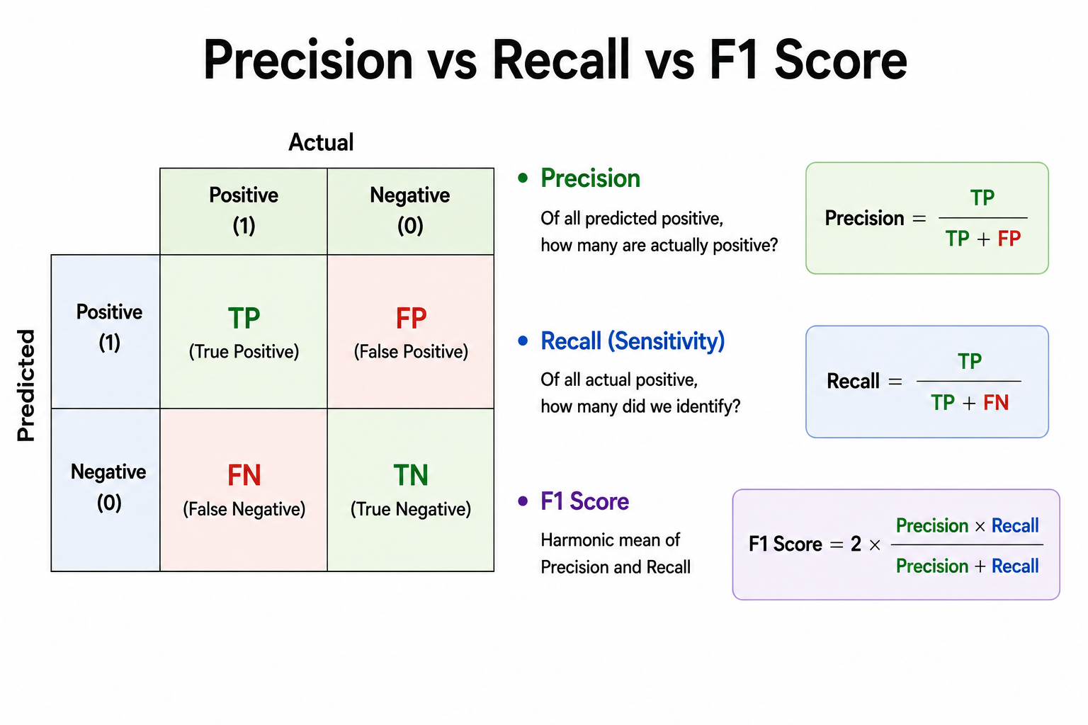
Precision:

•Measures how many predicted positives are truly positive.

•Focuses on reducing False Positives.

Precision = TP / (TP + FP)

Example: In spam detection, high precision means most emails flagged as spam are indeed spam.

Recall:

•Measures how many actual positives are correctly identified.

•Focuses on reducing False Negatives.

Recall = TP / (TP + FN)

Example: In disease diagnosis, high recall means most sick patients are detected.

Key Difference:

•Precision → accuracy of positive predictions (avoid false alarms).

•Recall → ability to find all positives (avoid missing cases).

F1-Score:

•Combines both precision and recall as their harmonic mean.

•Useful when both false positives and false negatives matter equally.

F1 = 2 × (Precision × Recall) / (Precision + Recall)

When to use which:

•Prioritize Precision → when false positives are costly (e.g., spam filter).

•Prioritize Recall → when false negatives are costly (e.g., cancer detection).

•Use F1-Score → when you need a balance of both.

How do precision and recall differ, and how does the F1 score combine these two metrics? image 1

Figure 7: ★ Precision, Recall, and F1-Score

What are some common loss functions used in machine learning?

GoogleAmazonMicrosoftMetaOpenAI

Solution

Mean Squared Error (MSE) — Regression:

•Penalizes larger errors by squaring them.

MSE = (1/n) × Σ(yᵢ - ŷᵢ)²

Mean Absolute Error (MAE) — Regression:

•Uses absolute differences; less sensitive to outliers than MSE.

MAE = (1/n) × Σ|yᵢ - ŷᵢ|

Huber Loss — Regression:

•Combines MSE and MAE; robust to outliers.

•Uses MSE for small errors, MAE for large ones.

Cross-Entropy Loss (Log Loss) — Classification:

•Measures the difference between predicted probabilities and actual labels.

Log Loss = -(1/n) × Σ[yᵢ × log(ŷᵢ) + (1 - yᵢ) × log(1 - ŷᵢ)]

Hinge Loss — SVM:

•Used in Support Vector Machines.

•Encourages maximum margin between classes.

KL Divergence — Probabilistic Models:

•Measures the difference between two probability distributions.

•Used in variational autoencoders and generative models.

Exponential Loss — Boosting:

•Used in AdaBoost; penalizes misclassified points strongly.

R-Squared (R²) — Regression:

•Indicates how well the model explains variance in the target variable.

•R² = 1 means perfect prediction; R² = 0 means no better than mean.

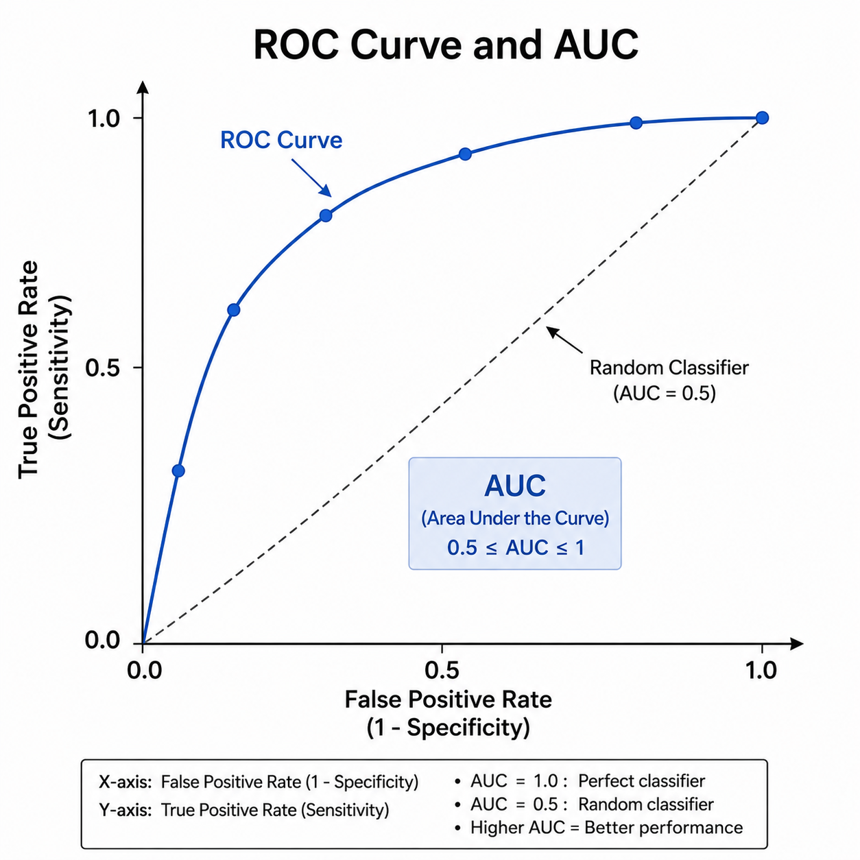
What is the AUC–ROC curve, and what does it represent?

GoogleAmazonMicrosoftMetaNetflix

Solution

ROC Curve (Receiver Operating Characteristic):

•Plots True Positive Rate (Recall) vs False Positive Rate at various classification thresholds.

TPR (Recall) = TP / (TP + FN)

FPR = FP / (FP + TN)

AUC (Area Under the Curve):

•Represents the probability that the model ranks a positive example higher than a negative example.

Interpretation:

•AUC = 1.0 → Perfect classifier — all positives ranked above all negatives.

•AUC = 0.5 → Random guessing — no discriminative ability.

•AUC < 0.5 → Worse than random — model predictions are inverted.

Why AUC-ROC is Useful:

•Threshold-independent — evaluates performance across all thresholds.

•Works well even with imbalanced datasets.

•Useful for comparing multiple models — higher AUC = better model.

Example:

•A model with AUC = 0.90 means there is a 90% chance the model ranks a diseased patient above a healthy one — strong discriminative ability.

What is the AUC–ROC curve, and what does it represent? image 1

Figure 9: ★ AUC-ROC Curve

Is accuracy always an appropriate metric for assessing classification models? Why or why not?

AmazonGoogleMicrosoftMetaApple

Solution

No, accuracy is not always an appropriate metric — especially with imbalanced datasets.

Why Accuracy Can Be Misleading:

•Consider a dataset with 95% negative and 5% positive samples.

•A model that always predicts "negative" achieves 95% accuracy but has completely failed — it never detects any positive case.

•This is known as the accuracy paradox.

Better Alternatives for Imbalanced Data:

Precision:

•How many predicted positives are actually positive.

•Important when false positives are costly (e.g., spam filter).

Precision = TP / (TP + FP)

Recall:

•How many actual positives were correctly identified.

•Important when false negatives are costly (e.g., disease detection).

Recall = TP / (TP + FN)

F1-Score:

•Harmonic mean of Precision and Recall.

•Best when you need a balance between both.

F1 = 2 × (Precision × Recall) / (Precision + Recall)

AUC-ROC:

•Evaluates model performance across all thresholds — ideal for imbalanced datasets.

Rule of Thumb:

•Use accuracy only when classes are roughly balanced.

•For imbalanced datasets, use F1-Score, Precision, Recall, or AUC-ROC.

What is Cross-Validation, and why is it important?

GoogleAmazonMicrosoftMetaNetflix

Solution

Cross-Validation tests how well a model generalizes by training and testing it multiple times on different data splits instead of relying on a single train-test split.

How it Works:

1. Split data into k folds (e.g., 5 or 10).

2. Train on k-1 folds, test on the remaining fold.

3. Repeat k times so each fold is used once as the test set.

4. Average all results for the final performance estimate.

CV Error = (1/k) × Σ errorᵢ

Types of Cross-Validation:

k-Fold:

•Dataset split into k equal folds.

•Most commonly used method.

Stratified k-Fold:

•Maintains class distribution in each fold.

•Useful for classification with imbalanced classes.

Leave-One-Out (LOO):

•k equals the number of samples.

•Each sample is used as the test set once.

•Very accurate but computationally expensive.

Hold-Out:

•Basic train-test split (e.g., 80/20).

•Fast but can be biased depending on the split.

Why Cross-Validation is Important:

•Reduces overfitting to a specific train-test split.

•Provides a more reliable performance estimate.

•Helps in model selection and hyperparameter tuning.

Can you explain k-Fold Cross-Validation, Leave-One-Out (LOO), and the Hold-Out method?

GoogleAmazonMicrosoftMetaApple

Solution

k-Fold Cross-Validation:

•Split dataset into k equal folds.

•Train on k-1 folds, test on 1 fold.

•Repeat k times so every fold is tested once.

•Average errors for final estimate.

CV Error = (1/k) × Σ errorᵢ

•Advantage: Reliable estimate with reduced variance.

•Disadvantage: Computationally heavier than hold-out.

Leave-One-Out (LOO):

•Special case of k-Fold where k = number of samples.

•Each individual data point is used as the test set once.

•All remaining samples are used for training.

•Advantage: Very accurate — uses maximum training data.

•Disadvantage: Very computationally expensive for large datasets.

Hold-Out Method:

•Simple split into training and testing sets.

•Common split: 70% train, 30% test or 80% train, 20% test.

•Advantage: Fast and simple to implement.

•Disadvantage: Prone to high variance — results depend heavily on which samples end up in each split.

When to Use Which:

•Hold-Out → Large datasets where speed matters.

•k-Fold → Medium datasets needing reliable evaluation.

•LOO → Small datasets where every data point is valuable.

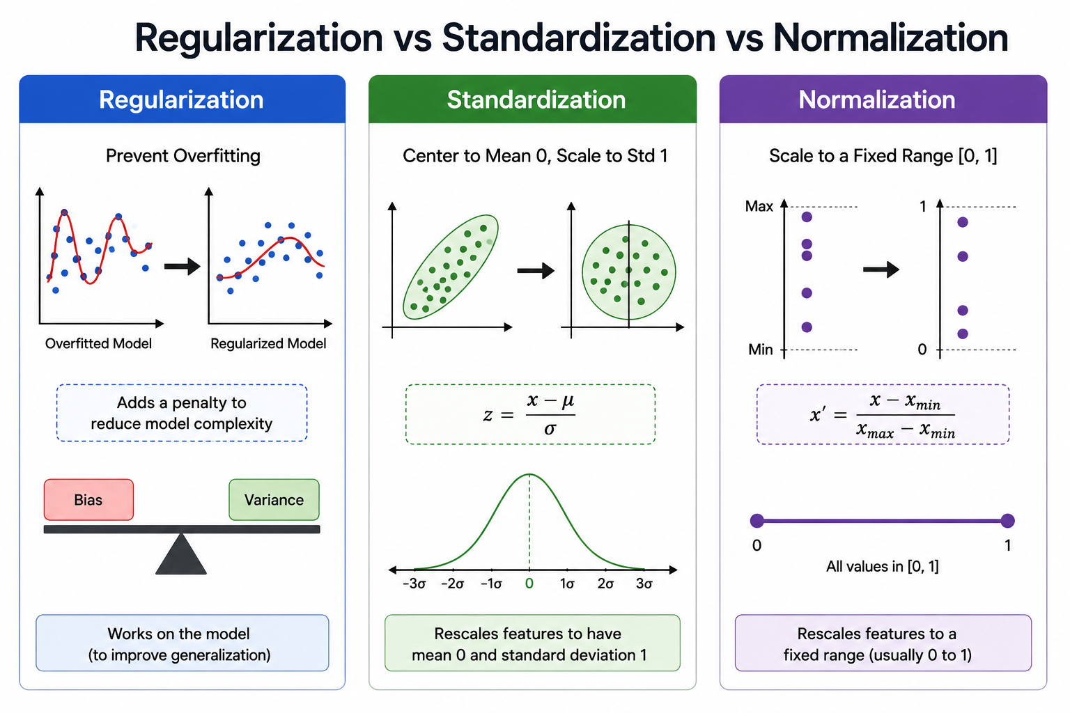
What distinguishes Regularization, Standardization, and Normalization from each other?

GoogleAmazonMicrosoftMetaNetflix

Solution

These three techniques are often confused but serve very different purposes:

Regularization:

•Purpose: Prevents overfitting by adding a penalty to the loss function.

•Applied to model training, not data preprocessing.

•Examples: L1 (Lasso), L2 (Ridge), Elastic Net, Dropout.

•Discourages large weights to simplify the model.

Standardization (Z-score Scaling):

•Purpose: Rescales features to have mean = 0 and standard deviation = 1.

x' = (x - mean) / std

•Used in scale-sensitive algorithms like SVM, KNN, Logistic Regression, PCA.

•Does not bound values to a fixed range.

•Preferred when data has outliers or does not follow a uniform distribution.

Normalization (Min-Max Scaling):

•Purpose: Rescales features into a fixed range, usually [0, 1].

x' = (x - x_min) / (x_max - x_min)

•Useful when features have different units or scales.

•Sensitive to outliers — one extreme value can compress all others.

•Preferred for algorithms like Neural Networks and KNN where input scale matters.

Quick Summary:

•Regularization → controls model complexity.

•Standardization → centers data around zero.

•Normalization → scales data to [0, 1].

What distinguishes Regularization, Standardization, and Normalization from each other? image 1

Figure 13: ★ Regularization, Standardization, and Normalization

What is Feature Engineering in the context of machine learning?

AmazonGoogleMicrosoftMetaNetflix

Solution

Feature Engineering is the process of creating, transforming, or selecting relevant features from raw data to improve model accuracy and generalization.

Key Steps in Feature Engineering:

Feature Creation:

•Generate new features from existing data.

•Example: Extract year, month, or day from a date column.

•Example: Create age from date of birth.

Feature Transformation:

•Apply scaling, normalization, or mathematical transforms.

•Common transforms: log, square root, Box-Cox.

•Used to handle skewed distributions or outliers.

Feature Encoding:

•Convert categorical variables to numeric representations.

•Methods: One-Hot Encoding, Label Encoding, Target Encoding.

Feature Selection:

•Keep only the most relevant features.

•Methods: Correlation, mutual information, model importance scores.

Handling Missing Data:

•Impute missing values using mean, median, mode, or prediction models.

Interaction Features:

•Combine two features to capture relationships.

•Example: Multiply price × quantity to get total revenue.

Why Feature Engineering Matters:

•Better features lead to better model performance.

•Reduces noise and irrelevant information.

•Can make a simple model outperform a complex one.

How does Feature Engineering differ from Feature Selection?

GoogleAmazonMicrosoftMetaApple

Solution

Feature Engineering and Feature Selection are both important preprocessing steps but serve different purposes:

Feature Engineering:

•Process of creating, transforming, or deriving new features from raw data to enhance model performance.

•Involves: creation, transformation, encoding, scaling, and combining features.

•Output: New or modified features added to the dataset.

•Example: Extracting Age from Date of Birth.

•Example: Generating sentiment score from raw text reviews.

Feature Selection:

•Process of choosing the most relevant features from the existing dataset to reduce noise and improve performance.

•Uses: correlation analysis, statistical tests, mutual information, or model importance scores.

•Output: A subset of the original features — no new features created.

•Example: Selecting the top 10 features from 50 using Random Forest importance scores.

Key Difference:

•Feature Engineering → Creates or transforms features (expands or modifies the feature space).

•Feature Selection → Filters features (reduces the feature space by removing irrelevant ones).

In Practice:

•Feature engineering is done first to create meaningful features.

•Feature selection is done after to remove redundant or irrelevant ones.

•Both steps together significantly improve model performance and reduce overfitting.

What are some common Feature Selection methods used in machine learning?

AmazonGoogleMicrosoftMetaNetflix

Solution

Feature selection methods are divided into three main categories:

Filter Methods:

•Assess features independently against the target variable using statistical tests — no ML model involved.

•Fast and scalable but ignores feature interactions.

Examples:

•Correlation Coefficient — measures linear relationship between feature and target.

•Chi-Square Test — for categorical features and classification targets.

•ANOVA F-Test — measures variance between groups.

•Mutual Information — measures dependency between feature and target.

Wrapper Methods:

•Evaluate subsets of features by training models and selecting the best combination.

•More accurate than filter methods but computationally expensive.

Examples:

•Forward Selection — starts with no features, adds one at a time.

•Backward Elimination — starts with all features, removes one at a time.

•Recursive Feature Elimination (RFE) — recursively removes least important features.

Embedded Methods:

•Feature selection occurs during model training — built into the algorithm.

•Efficient and considers feature interactions.

Examples:

•Lasso Regression (L1) — shrinks irrelevant feature weights to zero.

•Decision Tree / Random Forest importance scores — ranks features by their contribution to splits.

•Gradient Boosting feature importance — similar to Random Forest.

What is Dimensionality Reduction, and why is it used?

GoogleAmazonMicrosoftMetaApple

Solution

Dimensionality Reduction decreases the number of features (dimensions) in a dataset while retaining key information, leading to simpler models and better performance.

Why Dimensionality Reduction is Used:

Reduces Computation:

•Fewer features mean faster training and prediction.

•Critical for high-dimensional data (e.g., image pixels, text embeddings).

Enables Visualization:

•Reduces data to 2D or 3D for visual analysis.

•Helps identify patterns and clusters in data.

Removes Noise:

•Eliminates irrelevant or redundant features.

•Reduces overfitting by removing noise dimensions.

Addresses the Curse of Dimensionality:

•In high-dimensional spaces, data becomes sparse.

•Distance metrics become less meaningful — dimensionality reduction helps.

Common Techniques:

PCA (Principal Component Analysis):

•Linear technique that finds directions of maximum variance.

•Projects data onto fewer orthogonal components.

t-SNE (t-Distributed Stochastic Neighbor Embedding):

•Non-linear technique mainly used for visualization.

LDA (Linear Discriminant Analysis):

•Supervised technique that maximizes class separability.

Autoencoders:

•Neural network-based approach for non-linear dimensionality reduction.

Example:

•A dataset with 100 features reduced to 10 principal components capturing 95% of the variance.

What is Categorical Data, and how can it be processed?

AmazonGoogleMicrosoftMetaApple

Solution

Categorical Data represents discrete categories rather than continuous numbers.

Examples: Gender (Male/Female), Color (Red/Blue/Green), Product Type (Electronics/Clothing).

Types of Categorical Data:

Nominal (No Order):

•Categories have no meaningful order.

•Example: Color, Country, Brand.

Ordinal (Ordered):

•Categories have a meaningful ranking.

•Example: Low/Medium/High, Ratings (1-5 stars).

Encoding Techniques:

Label Encoding:

•Assigns a unique integer to each category.

•Example: Red=0, Blue=1, Green=2.

•Suitable for ordinal data where order matters.

•Risk: Can mislead models with nominal data by implying false ordering.

One-Hot Encoding:

•Converts categories into binary vectors with one column per category.

•Example: Red=[1,0,0], Blue=[0,1,0], Green=[0,0,1].

•Good for nominal data — avoids false ordering.

•Downside: Increases dimensionality for high-cardinality features.

Binary Encoding:

•Converts categories to binary code, reducing dimensionality compared to one-hot.

•Useful for high-cardinality features.

Target/Mean Encoding:

•Replaces categories with the mean of the target variable for that category.

•Powerful but can cause data leakage if not handled carefully.

What is the difference between label encoding and one-hot encoding?

GoogleAmazonMicrosoftMetaNetflix

Solution

Label Encoding:

•Maps each category to a unique integer.

•Example: Red=0, Blue=1, Green=2.

•Output: A single integer column.

Advantages:

•Simple and compact — no extra columns.

•Works well for ordinal data where order matters (e.g., Low=0, Medium=1, High=2).

Disadvantages:

•Can mislead models for nominal data by implying a false numerical relationship.

•Example: Model may think Green (2) > Blue (1) > Red (0) which is meaningless for colors.

One-Hot Encoding:

•Converts categories into binary vectors across multiple columns — one column per category.

•Example: Red=[1,0,0], Blue=[0,1,0], Green=[0,0,1].

•Output: N columns for N categories.

Advantages:

•Avoids false relationships between categories.

•Works well for nominal data (no inherent order).

Disadvantages:

•Increases dimensionality significantly for high-cardinality features.

•Can cause the curse of dimensionality with many unique categories.

When to Use Which:

•Label Encoding → Ordinal data (Low, Medium, High).

•One-Hot Encoding → Nominal data (Colors, Countries, Product Types).

•For high-cardinality nominal features, consider Target Encoding or Binary Encoding.

What do Upsampling and Downsampling mean in data processing?

AmazonGoogleMicrosoftMetaApple

Solution

Upsampling and downsampling are techniques to address imbalanced datasets where one class has significantly more samples than another.

Upsampling (Oversampling):

•Increases minority class samples to balance the dataset.

Methods:

•Random Oversampling: Duplicates existing minority samples randomly.

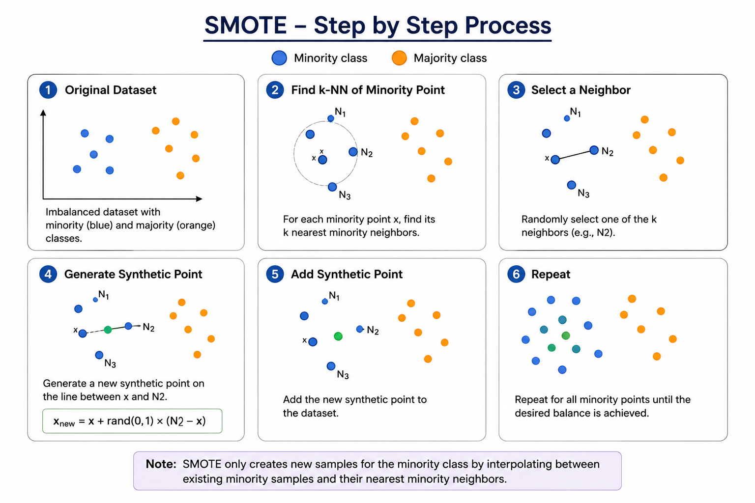
•SMOTE: Generates synthetic samples by interpolating between existing minority points.

Downsampling (Undersampling):

•Reduces majority class samples to balance the dataset.

Methods:

•Random Undersampling: Randomly removes majority class samples.

•Cluster-Based Undersampling: Removes samples based on clustering to maintain diversity.

Example:

•Dataset: 1000 positive samples, 100 negative samples (10:1 imbalance).

•Upsampling: Creates 900 extra minority (negative) samples → balanced 1000:1000.

•Downsampling: Reduces majority (positive) to 100 samples → balanced 100:100.

Trade-offs:

Upsampling:

•Preserves all original data.

•Risk of overfitting to duplicated minority samples.

Downsampling:

•Faster training with less data.

•Risk of losing important majority class information.

Best Practice:

•Use SMOTE for upsampling to generate diverse synthetic samples.

•Combine both techniques for best results.

How does the SMOTE technique address data imbalance issues?

GoogleAmazonMicrosoftMetaNetflix

Solution

SMOTE (Synthetic Minority Over-sampling Technique) creates synthetic minority samples by interpolating between existing minority class examples rather than simply duplicating them.

How SMOTE Works:

1. For each minority class sample, find its k nearest neighbors (typically k=5).

2. Randomly select one of those neighbors.

3. Generate a synthetic sample along the line segment between the original point and the selected neighbor.

Synthetic Point = Original + random(0,1) × (Neighbor - Original)

Why SMOTE is Better than Random Oversampling:

•Creates diverse, new synthetic samples instead of exact duplicates.

•The model trains on more varied examples — better generalization.

•Reduces the risk of overfitting compared to simple duplication.

Benefits:

•Balances class distribution without discarding majority data.

•Improves model performance on minority class detection.

•Works well for tabular, structured data.

Limitations:

•Overuse may introduce noise — synthetic points may overlap with majority class.

•Not ideal for high-dimensional or categorical data without modifications.

•Variants like Borderline-SMOTE and ADASYN address some limitations by focusing on borderline minority samples.

How does the SMOTE technique address data imbalance issues? image 1

Figure 21: ★ SMOTE Technique

What methods can be used to handle missing and duplicate data values?

AmazonGoogleMicrosoftMetaApple

Solution

Handling Missing Values:

Remove Rows or Columns:

•Drop rows with missing data if the amount is small.

•Drop entire columns if mostly missing (e.g., >50% missing).

Imputation:

•Mean/Median/Mode Imputation: Replace missing values with the column's mean (numerical), median (skewed), or mode (categorical).

•Forward/Backward Fill: Use the previous or next valid value — commonly used in time series data.

•Prediction-Based Imputation: Train a model to predict missing values using other features (e.g., KNN Imputer, regression).

Flag Missing:

•Add a binary indicator column marking whether a value was missing.

•Preserves the information that missingness itself may be meaningful.

Handling Duplicate Data:

Detection:

•Use `pandas df.duplicated()` to identify duplicate rows.

•Check for near-duplicates using fuzzy matching for text data.

Removal:

•Use `df.drop_duplicates()` to remove exact duplicate rows.

Smart Retention:

•Keep the most relevant row based on a timestamp, priority field, or recency.

•For partial duplicates, aggregate or merge the duplicate rows.

Why It Matters:

•Missing values can cause model errors or biased learning.

•Duplicates can artificially inflate model performance metrics.

What are outliers, and what approaches exist to manage them?

GoogleAmazonMicrosoftMetaNetflix

Solution

Outliers are data points that deviate significantly from the rest of the dataset. They may arise from measurement errors, data entry mistakes, or genuine rare events.

Detection Methods:

Box Plot / IQR Method:

•Points outside Q1 - 1.5×IQR or Q3 + 1.5×IQR are outliers.

•IQR = Q3 - Q1

Z-Score Method:

•Points with |z| > 3 are considered outliers.

•z = (x - mean) / std

Visualization:

•Scatter plots, histograms, and violin plots help visually identify outliers.

Handling Approaches:

Remove Outliers:

•Delete if caused by data entry errors or irrelevant to the problem.

•Only safe if outliers are truly erroneous.

Transform Data:

•Apply log or square root transformation to reduce skewness and compress extreme values.

Cap/Floor (Winsorization):

•Replace extreme values with defined upper and lower bounds.

•Example: Cap values at the 95th percentile.

Use Robust Models:

•Algorithms like Decision Trees and Random Forests are naturally resistant to outliers.

•Avoid linear regression for outlier-heavy data without transformation.

Keep Outliers:

•In fraud detection or anomaly detection, outliers are the target — keep and study them.

Can you explain the Bias-Variance tradeoff in machine learning?

GoogleAmazonMicrosoftMetaNetflix

Solution

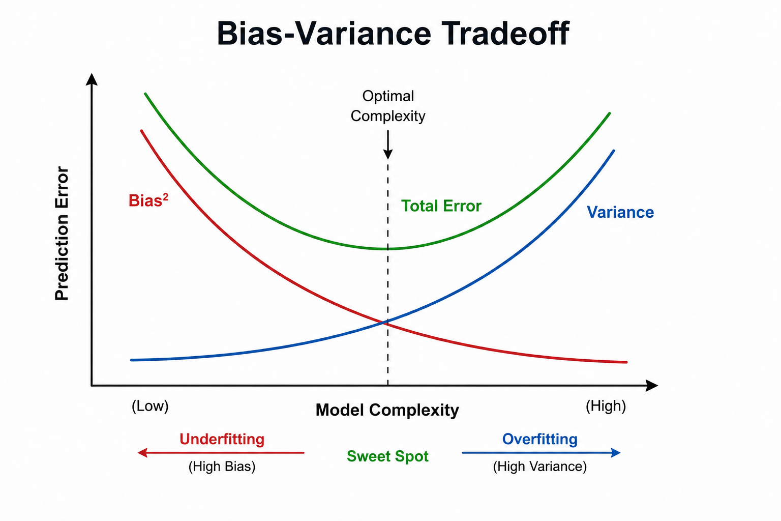
The Bias-Variance Tradeoff balances two types of errors that affect model performance.

Bias:

•Error from wrong assumptions in the model.

•High bias → model is too simple → underfitting.

•Example: Using linear regression for a non-linear problem.

•High bias models perform poorly on both training and test data.

Variance:

•Error from excessive sensitivity to training data fluctuations.

•High variance → model is too complex → overfitting.

•Example: A deep decision tree memorizing noise in training data.

•High variance models perform well on training but poorly on test data.

The Tradeoff:

•Reducing bias usually increases variance, and vice versa.

•The goal is to find the sweet spot that minimizes total error.

Total Error = Bias² + Variance + Irreducible Error

Irreducible Error:

•Noise in the data that cannot be removed regardless of model quality.

Visualizing the Tradeoff:

•Simple model (high bias, low variance) → underfits.

•Complex model (low bias, high variance) → overfits.

•Optimal model (balanced bias and variance) → generalizes well.

Solutions:

•High Bias → Use more complex model, add features, reduce regularization.

•High Variance → Use regularization, add more data, simplify model, use ensemble methods.

Can you explain the Bias-Variance tradeoff in machine learning? image 1

Figure 24: ★ Bias-Variance Tradeoff

What is Hyperparameter Tuning, and why is it necessary?

GoogleAmazonMicrosoftMetaApple

Solution

Hyperparameter Tuning finds the best hyperparameter values — settings that are configured before training begins — to maximize model performance.

Hyperparameters vs Parameters:

•Parameters (e.g., weights) are learned during training.

•Hyperparameters (e.g., learning rate, max depth, k in KNN) are set before training and control the training process.

Why It Is Necessary:

•Default hyperparameter values rarely produce optimal results.

•The right values can significantly improve accuracy and generalization.

•Poor hyperparameters can cause underfitting or overfitting.

Common Hyperparameter Tuning Methods:

Grid Search:

•Exhaustively tries all combinations of specified hyperparameter values.

•Thorough but very slow for large search spaces.

•Example: Try all combinations of learning_rate=[0.01, 0.1], max_depth=[3, 5, 7].

Random Search:

•Randomly samples combinations from the hyperparameter space.

•Faster than Grid Search and often finds equally good results.

•Better for large hyperparameter spaces.

Bayesian Optimization:

•Builds a probabilistic model of the relationship between hyperparameters and performance.

•Efficiently selects the next set of hyperparameters to evaluate.

•Balances exploration (trying new regions) and exploitation (refining promising regions).

•Most efficient method for expensive models.

What is Linear Regression, and what are its underlying assumptions?

GoogleAmazonMicrosoftMetaNetflix

Solution

Linear Regression is a supervised learning technique that fits a linear relationship to predict a continuous target variable based on one or more input features.

Formula:

y = mx + c

where y = predicted output, x = input feature, m = slope/coefficient, c = intercept.

For Multiple Features:

y = w₁x₁ + w₂x₂ + ... + wₙxₙ + b

Types:

•Simple Linear Regression — one input feature.

•Multiple Linear Regression — multiple input features.

Assumptions of Linear Regression:

Linearity:

•There must be a linear relationship between the input features and the target variable.

Independence:

•Data points are independent of each other — no autocorrelation.

Homoscedasticity:

•Error terms have constant variance across all levels of the independent variable.

•Violation causes unreliable confidence intervals.

Normality of Errors:

•Residuals (errors) should follow a normal distribution.

No Multicollinearity:

•Input features should not be highly correlated with each other.

•Multicollinearity makes it hard to interpret individual feature effects.

Why Assumptions Matter:

•Violations can lead to unreliable coefficients and predictions.

•Always validate assumptions using residual plots, VIF, and statistical tests.

How does the sigmoid function operate within Logistic Regression?

GoogleAmazonMicrosoftMetaApple

Solution

In Logistic Regression, the sigmoid function converts any real-valued number into a value between 0 and 1, making it suitable for representing probabilities.

Sigmoid Formula:

σ(z) = 1 / (1 + e^(-z))

where z = w₁x₁ + w₂x₂ + ... + wₙxₙ + b (the linear combination of inputs).

Properties of the Sigmoid Function:

•Output always between 0 and 1.

•σ(z) → 1 as z → +∞

•σ(z) → 0 as z → -∞

•σ(0) = 0.5 (decision boundary)

How It Works in Logistic Regression:

1. Compute the linear combination z = wx + b.

2. Pass z through the sigmoid function to get a probability p = σ(z).

3. Apply a threshold (typically 0.5):

- If p ≥ 0.5 → predict class 1.

- If p < 0.5 → predict class 0.

Important Distinction:

•Despite being called "regression," Logistic Regression is used for classification, not predicting continuous values.

•It predicts the probability of belonging to a class, then applies a threshold.

Use Cases:

•Binary classification: spam/not-spam, disease/no-disease, fraud/no-fraud.

How can one determine the optimal number of clusters in clustering algorithms?

AmazonGoogleMicrosoftMetaNetflix

Solution

Choosing the right number of clusters (K) is critical for meaningful results. Common methods include:

Elbow Method:

•Plot Within-Cluster Sum of Squares (WCSS) or explained variance versus the number of clusters.

•The point where the curve bends like an elbow (rate of improvement slows) indicates the optimal K.

•Simple and widely used but sometimes subjective.

WCSS = Σ Σ ||xᵢ - μⱼ||²

Silhouette Score:

•Measures how similar each point is to its own cluster vs other clusters.

•Score ranges from -1 to +1 — higher is better.

•The K with the highest average silhouette score is optimal.

Silhouette = (b - a) / max(a, b)

where a = mean intra-cluster distance, b = mean nearest-cluster distance.

Gap Statistic:

•Compares within-cluster dispersion to a reference random clustering of the same data.

•The optimal K has the largest gap between actual and expected dispersion.

•More statistically rigorous than the elbow method.

Dendrogram (Hierarchical Clustering):

•A tree diagram showing how clusters merge.

•Cut the dendrogram at the longest vertical line that doesn't cross any horizontal lines.

Domain Knowledge:

•Sometimes the business problem dictates the number of clusters.

•Example: A retail company may want exactly 5 customer segments.

What is Multicollinearity, and why does it pose a problem?

GoogleAmazonMicrosoftMetaApple

Solution

Multicollinearity occurs when two or more independent features are highly correlated with each other in a regression model.

Problems Caused by Multicollinearity:

Unstable Coefficients:

•Small changes in data cause large swings in coefficients.

•Makes the model unreliable and hard to interpret.

Difficult Interpretation:

•Hard to isolate the individual effect of each feature on the target.

•Coefficients may even have the wrong sign.

Inflated Standard Errors:

•High standard errors reduce the statistical significance of features.

•Important features may appear insignificant.

Reduced Model Explainability:

•Cannot determine which correlated feature is truly driving predictions.

Detection Methods:

Correlation Matrix:

•High correlation (|r| > 0.8) between two features signals multicollinearity.

Variance Inflation Factor (VIF):

•VIF > 5 indicates moderate multicollinearity.

•VIF > 10 indicates severe multicollinearity.

Solutions:

•Remove one of the highly correlated features.

•Combine correlated features (e.g., create a composite feature).

•Apply PCA to transform correlated features into independent components.

•Use Ridge Regression (L2) which handles multicollinearity by shrinking coefficients.

What is the Variance Inflation Factor (VIF)?

GoogleAmazonMicrosoftMetaNetflix

Solution

Variance Inflation Factor (VIF) quantifies how much a coefficient's variance is inflated due to correlations with other features in a regression model.

Formula:

VIF_i = 1 / (1 - R_i²)

where R_i² is the R-squared value from regressing feature i on all other features.

Interpretation:

•VIF = 1 → No correlation with other features. Perfect.

•1 < VIF < 5 → Moderate correlation. Generally acceptable.

•VIF > 5 → High multicollinearity. Concerning — investigate further.

•VIF > 10 → Severe multicollinearity. Must address before using the model.

How to Calculate VIF:

1. For each feature i, regress it against all other features.

2. Record the R² value.

3. Apply the formula: VIF = 1 / (1 - R²).

4. Features with high VIF are highly explained by others — candidates for removal.

How to Handle High VIF:

•Remove one of the correlated features.

•Combine correlated features into one (e.g., average or PCA).

•Apply Ridge Regression which is robust to multicollinearity.

Why VIF Matters:

•High VIF means the model coefficient estimates are unreliable and unstable.

•Even a small change in data can drastically change the coefficient values.

How are Information Gain and Entropy used in Decision Trees?

AmazonGoogleMicrosoftMetaApple

Solution

Entropy measures the impurity or disorder in a dataset. A node is pure when all samples belong to one class.

Entropy Formula:

Entropy(S) = -Σ pᵢ × log₂(pᵢ)

where pᵢ is the proportion of samples belonging to class i.

Entropy Values:

•Entropy = 0 → Completely pure node (all one class).

•Entropy = 1 → Maximum disorder (classes equally mixed).

Information Gain measures the reduction in entropy when the dataset is split by a feature. A higher information gain means a better split.

Information Gain Formula:

IG(S, A) = Entropy(S) - Σ (|Sᵥ| / |S|) × Entropy(Sᵥ)

where S is the dataset, A is the feature, and Sᵥ are the subsets after splitting by feature A.

How Decision Trees Use These:

1. Calculate entropy of the current node.

2. For each feature, calculate the information gain of splitting by that feature.

3. Select the feature with the highest information gain.

4. Split the node and repeat recursively.

Example:

•If splitting by "Color" reduces entropy from 1.0 to 0.3, the information gain is 0.7.

•If splitting by "Size" reduces entropy to 0.6, the information gain is 0.4.

•Decision tree picks Color as it gives higher information gain.

What techniques can help prevent overfitting in Decision Trees?

GoogleAmazonMicrosoftMetaNetflix

Solution

Decision trees are prone to overfitting because they can grow very deep and fit noise as well as patterns. Here are effective prevention techniques:

Limit Tree Depth:

•Set a max_depth parameter to stop the tree from growing too deep.

•Shallower trees are simpler and generalize better.

Minimum Samples for Splits:

•Set min_samples_split — minimum number of samples required to split a node.

•Prevents splitting on very small subsets that may just be noise.

Minimum Samples for Leaves:

•Set min_samples_leaf — minimum number of samples a leaf node must have.

•Avoids creating leaf nodes representing only 1-2 samples.

Pruning:

•Pre-Pruning (Early Stopping): Stop tree growth early using constraints like max_depth.

•Post-Pruning: Grow the full tree then remove branches with minimal impact on accuracy.

Use Relevant Features:

•Limit the number of features considered at each split using max_features.

•Avoids using irrelevant features for splits.

Ensemble Methods:

•Random Forest — builds many trees on random subsets and averages results.

•Gradient Boosting — builds trees sequentially to correct errors.

•Both significantly reduce variance compared to a single decision tree.

Cross-Validation:

•Monitor performance on validation data to detect overfitting early.

What does Pruning mean in the context of Decision Trees?

AmazonGoogleMicrosoftMetaApple

Solution

Pruning removes branches from a decision tree that do not add significant predictive power, making the tree simpler, faster, and less prone to overfitting.

Why Pruning is Needed:

•Unpruned trees grow until every training sample is correctly classified.

•This causes severe overfitting — the tree memorizes noise.

•Pruning trades a small increase in training error for a large reduction in test error.

Types of Pruning:

Pre-Pruning (Early Stopping):

•Stop tree growth before it fully fits the training data.

•Controlled by setting constraints:

- max_depth — maximum depth of the tree.

- min_samples_split — minimum samples needed to split a node.

- min_samples_leaf — minimum samples required in a leaf node.

•Simple and fast but may stop tree growth too early.

Post-Pruning:

•Grow the full tree first, then remove branches with little impact on accuracy.

•More accurate than pre-pruning since it sees the full tree before deciding.

Cost Complexity Pruning (CCP):

•Balances accuracy and tree size using a penalty term alpha (α).

•Higher alpha → more aggressive pruning → simpler tree.

•Lower alpha → less pruning → more complex tree.

•Choose optimal alpha using cross-validation.

Benefit:

•Pruned trees are more interpretable and generalize better to unseen data.

Can you explain the ID3 and CART algorithms?

GoogleAmazonMicrosoftMetaNetflix

Solution

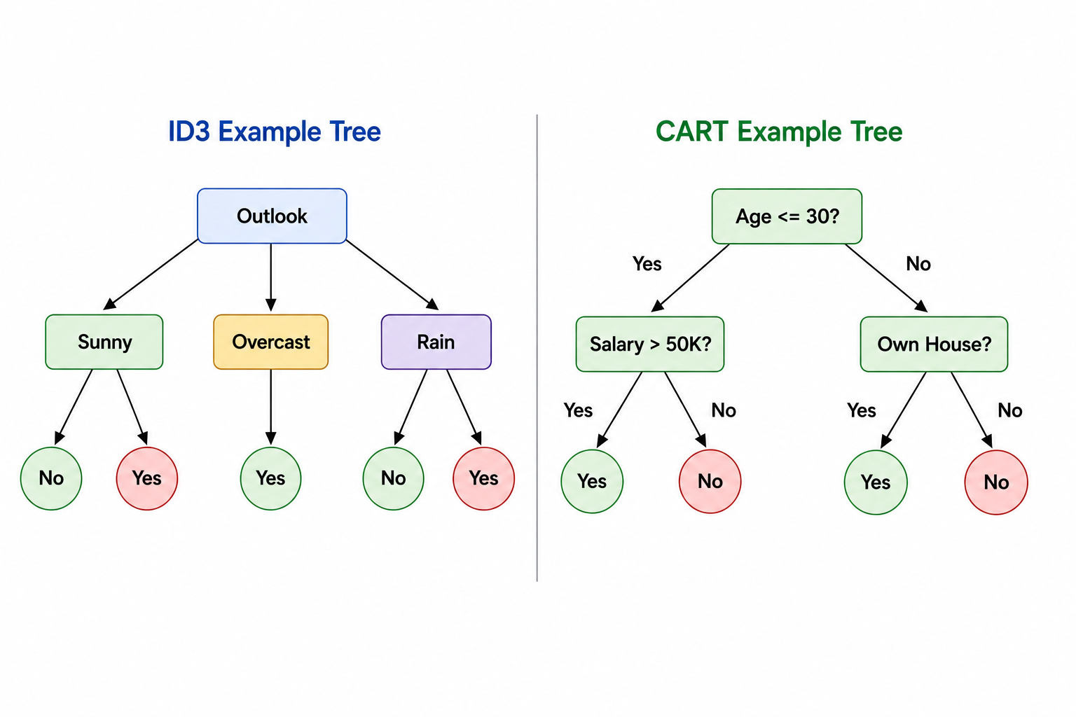
ID3 (Iterative Dichotomiser 3):

•A classic decision tree algorithm for classification only.

•Uses Entropy and Information Gain to select the best feature for splitting.

ID3 Steps:

1. Calculate entropy of the current dataset.

2. Compute information gain for each feature.

3. Select the feature with highest information gain.

4. Split the dataset and repeat recursively.

5. Stop when a node is pure or no features remain.

ID3 Characteristics:

•Classification only — no regression support.

•Supports multi-way splits (one branch per category value).

•Primarily handles categorical data.

•Does not have built-in pruning.

CART (Classification and Regression Trees):

•A versatile algorithm supporting both classification and regression.

•Uses Gini Index for classification and Mean Squared Error (MSE) for regression.

CART Characteristics:

•Always forms binary trees (splits into exactly two branches).

•Handles both numeric and categorical data.

•Supports cost complexity pruning to prevent overfitting.

•Foundation for ensemble methods like Random Forest and Gradient Boosting.

Key Differences:

•ID3 → Classification only, multi-way splits, entropy/information gain, mainly categorical.

•CART → Classification and regression, binary splits, Gini/MSE, numeric and categorical data.

Can you explain the ID3 and CART algorithms? image 1

Figure 34: ★ ID3 vs CART

What is Naive Bayes, and how does Bayes' Theorem apply to it?

GoogleAmazonMicrosoftMetaApple

Solution

Bayes' Theorem calculates the probability of an event based on prior knowledge of related conditions.

Bayes' Theorem Formula:

P(A|B) = [P(B|A) × P(A)] / P(B)

where:

•P(A|B) = Posterior — probability of A given B occurred.

•P(B|A) = Likelihood — probability of B given A is true.

•P(A) = Prior — initial probability of A.

•P(B) = Evidence — total probability of B.

Naive Bayes Classifier:

•A classification algorithm that applies Bayes' Theorem with the "naive" assumption that all features are conditionally independent given the class label.

•Despite this oversimplification, it works surprisingly well in practice.

How Naive Bayes Works:

1. Calculate prior probabilities for each class from training data.

2. Compute likelihoods of each feature value per class.

3. Apply Bayes' theorem to compute posterior probabilities.

4. Assign the class with the highest posterior probability.

Common Applications:

•Spam detection — classify emails as spam or not.

•Weather forecasting — predict weather based on conditions.

•Sentiment analysis — classify text as positive or negative.

•Medical diagnosis — predict disease based on symptoms.

Why "Naive":

•The independence assumption is rarely true in real data — hence "naive."

•Yet the algorithm often performs well due to its simplicity and fast computation.

What are the different types of Naive Bayes algorithms?

GoogleAmazonMicrosoftMetaNetflix

Solution

There are four main types of Naive Bayes algorithms, each suited for different data distributions:

Gaussian Naive Bayes:

•Assumes continuous features follow a normal (Gaussian) distribution.

•Used when features are real-valued continuous numbers.

•Examples: Height, weight, temperature, age.

•Calculates likelihood using the Gaussian probability density function.

Multinomial Naive Bayes:

•Works with discrete count data.

•Most commonly used for text classification where features represent word counts or frequencies.

•Examples: Document classification, spam filtering with word frequency features.

Bernoulli Naive Bayes:

•Suitable for binary features — each feature is either 0 or 1.

•Used in text classification where features represent word presence/absence (not count).

•Example: Email spam detection based on whether specific words appear.

Categorical Naive Bayes:

•Used when features are categorical (discrete unordered values).

•Example: Classifying based on Color (Red/Blue/Green) or Day of Week.

Choosing the Right Type:

•Continuous numeric features → Gaussian Naive Bayes.

•Word counts / frequency data → Multinomial Naive Bayes.

•Binary/boolean features → Bernoulli Naive Bayes.

•Categorical features → Categorical Naive Bayes.

How does the K-Nearest Neighbors (KNN) algorithm function?

AmazonGoogleMicrosoftMetaApple

Solution

K-Nearest Neighbors (KNN) is a simple, non-parametric supervised learning algorithm used for both classification and regression. It predicts based on the majority class or average value of the K nearest neighbors.

How KNN Works:

1. Choose K — the number of nearest neighbors to consider.

2. Compute distances from the query point to all training points using a distance metric (typically Euclidean distance).

3. Select K nearest neighbors — the K training points with the smallest distances.

4. Make prediction:

- Classification → Assign the most frequent class among K neighbors (majority vote).

- Regression → Assign the average value of K neighbors.

Distance Formula (Euclidean):

d(p, q) = √(Σ(pᵢ - qᵢ)²)

Key Characteristics:

•Non-parametric — makes no assumptions about data distribution.

•Lazy learner — no explicit training phase; all computation at prediction time.

•Simple but powerful for low-dimensional data.

Common Distance Metrics:

•Euclidean distance (most common).

•Manhattan distance.

•Minkowski distance.

Hyperparameters:

•K — number of neighbors (tuned via cross-validation).

•Distance metric — affects which neighbors are selected.

Why is KNN categorized as a lazy learning algorithm?

GoogleAmazonMicrosoftMetaNetflix

Solution

KNN is called a lazy learning algorithm because it does not build a model during the training phase. Instead, it simply stores all the training data and defers all computation to prediction time.

What "Lazy" Means:

No Training Phase:

•Unlike algorithms like linear regression or decision trees that learn a model during training, KNN does nothing during training.

•It just memorizes the entire training dataset.

Computation at Prediction Time:

•When a new query point arrives, KNN computes distances to all stored training points.

•It selects K nearest neighbors and makes the prediction.

•All the "work" happens at query time, not training time.

Consequences of Lazy Learning:

Memory Intensive:

•Must store all training data in memory.

•Large datasets require significant storage.

Slow Prediction:

•Computing distances to all training points for every prediction can be very slow for large datasets.

•Time complexity: O(n × d) per prediction where n = samples, d = dimensions.

Fast "Training":

•"Training" is instantaneous since no model is built.

Contrast with Eager Learners:

•Eager learners (e.g., Decision Trees, SVM) build a model during training and make fast predictions.

•Lazy learners (KNN) skip training but pay the cost at prediction time.

How does the choice of K value impact KNN performance?

AmazonGoogleMicrosoftMetaApple

Solution

The choice of K is one of the most important hyperparameters in KNN and directly impacts model performance.

Small K (e.g., K=1 or K=3):

•Model is sensitive to noise in training data.

•Decision boundaries are irregular and complex.

•Tends to overfit — performs well on training data but poorly on test data.

•Single outliers can drastically change predictions.

Large K (e.g., K=50 or K=100):

•Smooths decision boundaries by considering more neighbors.

•Can underfit — ignores important local patterns in data.

•Predictions become dominated by the overall majority class.

•Computationally more expensive.

Optimal K:

•Balances overfitting and underfitting.

•Typically chosen using cross-validation — test multiple K values and pick the one with best validation performance.

•A common rule of thumb: K = √n where n is the number of training samples.

•Odd values of K are preferred for binary classification to avoid ties.

Effect Summary:

•K too small → High variance, overfitting.

•K too large → High bias, underfitting.

•K optimal → Best generalization.

Practical Tip:

•Plot the error rate vs K curve and choose K at the elbow where test error is minimized.

What is meant by the decision boundary in Support Vector Machines (SVM)?

GoogleAmazonMicrosoftMetaApple

Solution

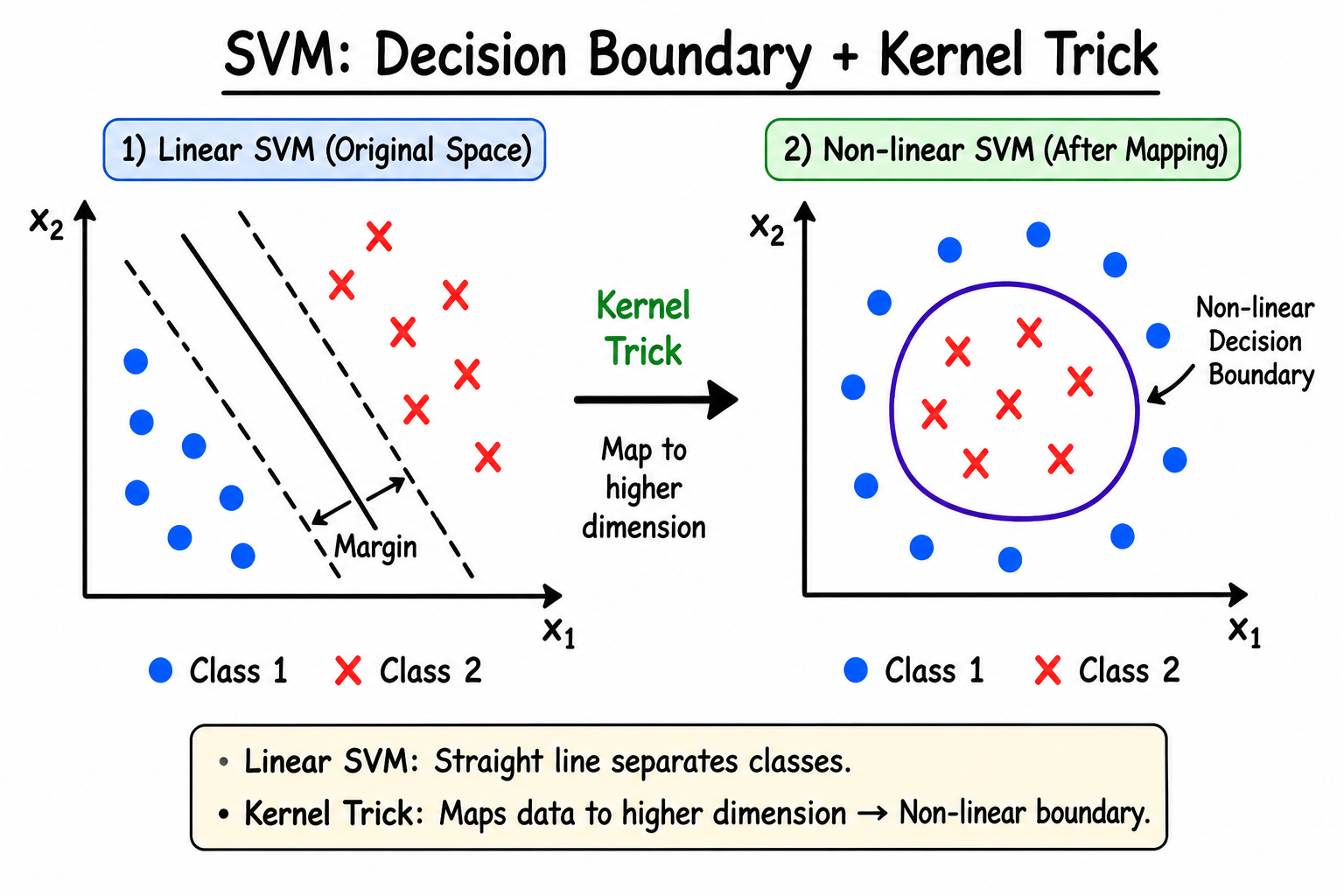
In Support Vector Machine (SVM), the decision boundary is the line (in 2D), plane (in 3D), or hyperplane (in higher dimensions) that separates different classes in the feature space.

Key Concepts:

Hyperplane:

•The decision boundary that divides the feature space into class regions.

•In 2D: a line. In 3D: a plane. In n dimensions: a hyperplane.

Equation of the Hyperplane:

w·x + b = 0

where w = weight vector, x = input features, b = bias.

Margin:

•The distance between the hyperplane and the nearest data points from each class.

•These nearest points are called Support Vectors.

•SVM maximizes this margin for better generalization.

Maximum Margin Classifier:

•SVM finds the hyperplane that maximizes the margin between classes.

•A larger margin means the model is more confident and generalizes better.

Support Vectors:

•The critical data points closest to the decision boundary.

•They define and support the hyperplane — removing other points wouldn't change the boundary.

Hard vs Soft Margin:

•Hard Margin SVM: No misclassification allowed — requires perfectly separable data.

•Soft Margin SVM: Allows some misclassification using a penalty parameter C to handle noisy or non-separable data.

What is the kernel trick in SVM, and why is it useful?

GoogleAmazonMicrosoftMetaNetflix

Solution

The kernel trick in SVM enables handling non-linearly separable data by implicitly mapping it to a higher-dimensional space where it becomes linearly separable — without ever explicitly computing the transformation.

Why It's Needed:

•In the original feature space, some data cannot be separated by a straight line.

•By projecting data to a higher dimension, a linear hyperplane can separate the classes.

•The kernel trick avoids the expensive computation of explicitly transforming data.

How It Works:

•Instead of computing the actual high-dimensional coordinates, the kernel function computes the dot product in the transformed space directly.

K(x, y) = φ(x) · φ(y)

where φ is the mapping function and K is the kernel function.

Common Kernels:

Linear Kernel:

•K(x, y) = xᵀy

•For linearly separable data; fast and simple.

Polynomial Kernel:

•K(x, y) = (xᵀy + c)^d

•For polynomial feature relationships.

RBF (Radial Basis Function) / Gaussian Kernel:

•K(x, y) = exp(-γ||x - y||²)

•For complex non-linear data; most widely used kernel.

Sigmoid Kernel:

•K(x, y) = tanh(αxᵀy + c)

•Similar to neural networks; less common than RBF.

Why the Kernel Trick is Powerful:

•Enables SVM to solve non-linear problems efficiently.

•No need to manually engineer polynomial features.

What is the kernel trick in SVM, and why is it useful? image 1

Figure 41: ★ Kernel Trick in SVM

What is Ensemble Learning in machine learning?

AmazonGoogleMicrosoftMetaNetflix

Solution

Ensemble Learning combines multiple models (weak learners) to create a stronger, more accurate model by aggregating their predictions.

Core Idea:

•A single model may be biased or overfit.

•Combining many models averages out errors and improves overall accuracy.

•"The wisdom of the crowd" applied to machine learning.

Why It Works:

•Individual models make different errors.

•When combined, errors cancel out and correct predictions are reinforced.

Main Ensemble Techniques:

Bagging (Bootstrap Aggregating):

•Builds multiple models in parallel on random subsets of data (with replacement).

•Combines outputs by voting (classification) or averaging (regression).

•Reduces variance — prevents overfitting.

•Example: Random Forest.

Boosting:

•Trains models sequentially, each correcting the previous model's errors.

•Combines models weighted by their accuracy.

•Reduces bias — improves accuracy on hard examples.

•Examples: AdaBoost, XGBoost, Gradient Boosting.

Stacking:

•Combines predictions of multiple base models via a meta-model (blender).

•Meta-model learns how to best combine base model predictions.

Voting:

•Combines results by majority vote (classification) or averaging (regression).

•Simple but effective when models are diverse.

Could you explain the concepts of Bagging and Boosting?

GoogleAmazonMicrosoftMetaNetflix

Solution

Bagging (Bootstrap Aggregating):

•Trains multiple models in parallel on different random subsets of training data (sampled with replacement — bootstrapping).

•Each model is independent of the others.

•Final prediction: majority vote (classification) or average (regression).

•Primarily reduces variance — prevents overfitting.

•Example: Random Forest builds many decision trees using bagging.

Boosting:

•Trains models sequentially — each new model focuses on correcting the mistakes of the previous model.

•Misclassified samples are given higher weights so the next model focuses on them.

•Final prediction: weighted combination of all models (weights based on accuracy).

•Primarily reduces bias — improves performance on difficult examples.

•Can overfit if unchecked.

•Examples: AdaBoost, Gradient Boosting, XGBoost.

Key Differences:

Training:

•Bagging → parallel (models trained independently).

•Boosting → sequential (each model depends on previous).

Goal:

•Bagging → reduces variance.

•Boosting → reduces bias.

Overfitting:

•Bagging → less prone to overfitting.

•Boosting → can overfit if too many rounds.

Speed:

•Bagging → faster (parallelizable).

•Boosting → slower (sequential).

What characterizes a Random Forest model?

AmazonGoogleMicrosoftMetaNetflix

Solution

Random Forest is an ensemble learning algorithm that builds multiple decision trees on bootstrapped subsets of data and combines their results via majority vote or averaging to improve accuracy and stability.

How Random Forest Works:

1. Create bootstrapped data subsets (random samples with replacement).

2. Build a decision tree for each subset using a random subset of features at each split.

3. Each tree makes independent predictions.

4. Final prediction:

- Classification → majority vote across all trees.

- Regression → average of all tree outputs.

Key Advantages:

Higher Accuracy:

•More accurate than a single decision tree on large datasets.

•Averaging many trees reduces noise.

Reduces Overfitting:

•Aggregating many trees averages out variance.

•Random feature selection at each split decorrelates trees.

Handles Mixed Data:

•Works with both categorical and numerical features.

Feature Importance:

•Provides built-in feature importance scores based on how much each feature reduces impurity across all trees.

Robust to Outliers:

•Decision trees are naturally robust to outliers — Random Forest inherits this.

Disadvantages:

•Less interpretable than a single decision tree.

•Slower prediction — must query all trees.

•Memory intensive — stores all trees.

How do AdaBoost, XGBoost, and CatBoost algorithms work?

GoogleAmazonMicrosoftMetaNetflix

Solution

AdaBoost (Adaptive Boosting):

•Combines multiple weak learners (typically shallow decision trees — depth 1 "stumps").

•After each round, misclassified samples get higher weights so the next learner focuses on them.

•Final prediction is a weighted majority vote — better learners get more weight.

•Best for improving simple models on clean data.

•Sensitive to noisy data and outliers.

XGBoost (Extreme Gradient Boosting):

•An optimized gradient boosting implementation.

•Builds trees sequentially, each correcting prior errors using gradient descent on the loss function.

•Key features:

- L1 and L2 regularization — prevents overfitting.

- Handles missing values natively.

- Parallelizable — fast despite sequential tree building.

- Pruning using max_depth and min_child_weight.

•Best for structured/tabular data — consistently top performer on Kaggle competitions.

CatBoost (Categorical Boosting):

•Gradient boosting designed specifically to handle categorical features without heavy preprocessing.

•Uses ordered boosting to reduce prediction shift and overfitting.

•Encodes categorical features automatically during training.

•Key advantages:

- Requires less tuning than XGBoost.

- Excellent with datasets having many categorical features.

- Minimal data preprocessing needed.

Can you describe the K-Means Clustering algorithm?

AmazonGoogleMicrosoftMetaNetflix

Solution

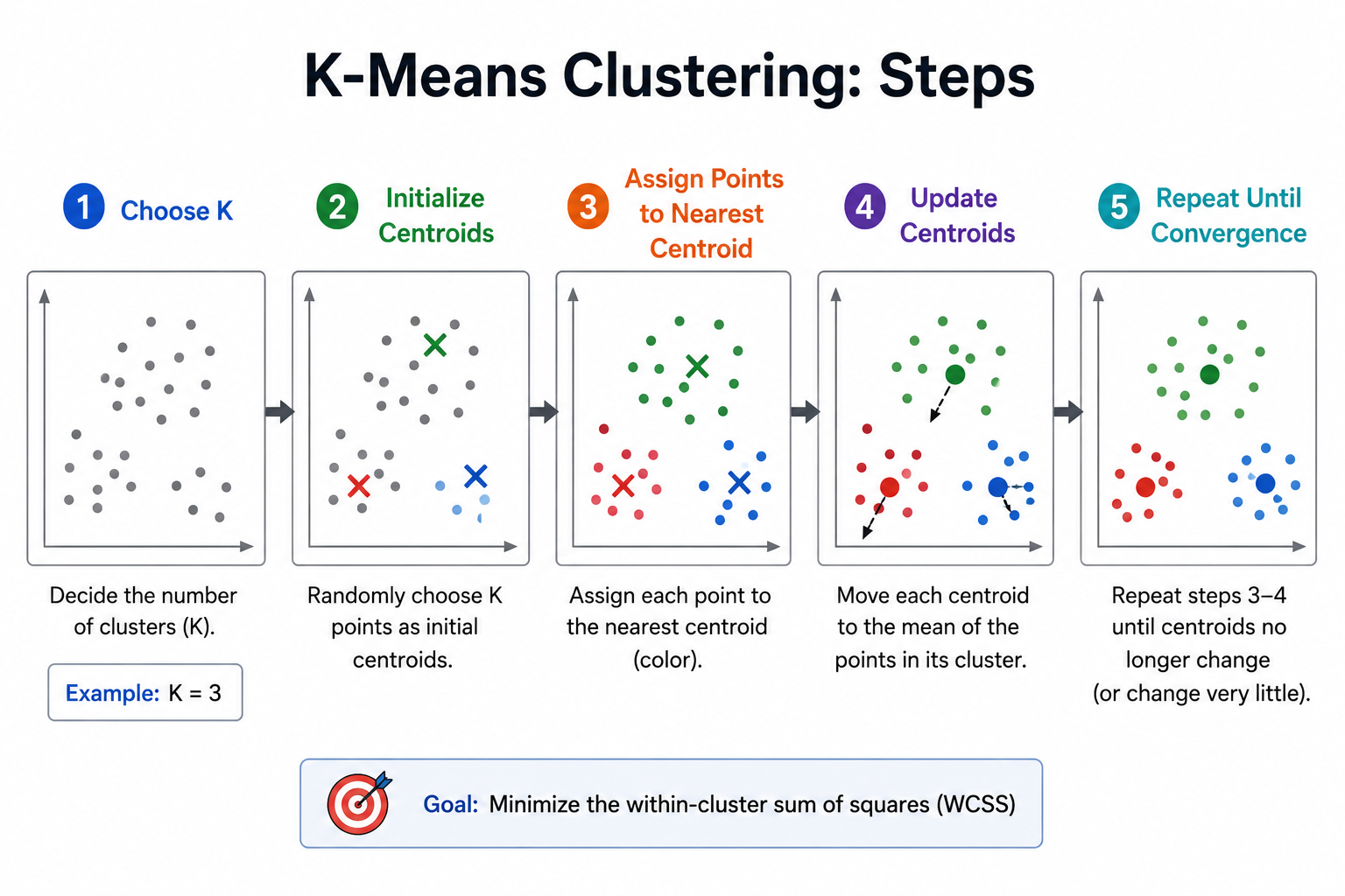
K-Means Clustering is an unsupervised machine learning algorithm that groups similar data points into K clusters by minimizing the distance between points and their cluster centroid.

How K-Means Works:

1. Select K — choose the number of clusters.

2. Initialize K centroids randomly from the dataset.

3. Assign each point to the nearest centroid using Euclidean distance.

4. Recalculate centroids — new centroid = mean of all points in the cluster.

5. Repeat steps 3 and 4 until centroids stabilize (convergence).

Objective — Minimize WCSS:

WCSS = Σ Σ ||xᵢ - μⱼ||²

where xᵢ is each data point and μⱼ is the centroid of cluster j.

Advantages:

•Simple and fast — computationally efficient.

•Suitable for large datasets.

•Easy to interpret and visualize.

Disadvantages:

•Must specify K in advance — K is not learned automatically.

•Sensitive to outliers — outliers pull centroids away from true cluster centers.

•Can converge to local minima — results depend on initial centroid placement.

•Assumes spherical, similarly-sized clusters — struggles with irregular shapes.

Choosing K:

•Use the Elbow Method or Silhouette Score to find the optimal K.

Can you describe the K-Means Clustering algorithm? image 1

Figure 46: ★ Choosing the Right K in K-Means

What is Hierarchical Clustering, and how does it work?

GoogleAmazonMicrosoftMetaApple

Solution

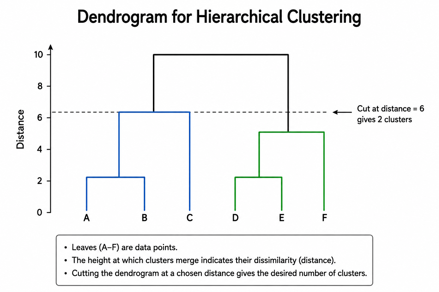
Hierarchical Clustering is an unsupervised method that groups data points by building a hierarchy of clusters (tree structure). The result is visualized as a dendrogram.

Types of Hierarchical Clustering:

Agglomerative (Bottom-Up) — Most Common:

1. Start with each data point as its own cluster.

2. Find the two closest clusters using a linkage criterion.

3. Merge those two clusters into one.

4. Repeat until only one cluster remains.

Divisive (Top-Down):

1. Start with all points in one cluster.

2. Recursively split clusters based on dissimilarity.

3. Continue until each point is its own cluster.

Linkage Criteria (how to measure cluster distance):

•Single Linkage — minimum distance between any two points in clusters.

•Complete Linkage — maximum distance between any two points.

•Average Linkage — average distance between all point pairs.

•Ward's Method — minimizes total within-cluster variance (most popular).

Dendrogram:

•Tree diagram showing the merging history of clusters.

•Cut the dendrogram at a chosen height to obtain K clusters.

Advantages:

•No need to specify K in advance — choose by cutting the dendrogram.

•Provides visual insight into cluster structure.

Disadvantages:

•Computationally expensive — O(n³) for large datasets.

•Sensitive to noise and outliers.

What is Hierarchical Clustering, and how does it work? image 1

Figure 47: ★ Hierarchical Clustering

How does the DBSCAN clustering algorithm function?

GoogleAmazonMicrosoftMetaNetflix

Solution

DBSCAN (Density-Based Spatial Clustering of Applications with Noise) is an unsupervised clustering algorithm that groups points based on density, not distance — making it ideal for clusters of arbitrary shape.

Key Parameters:

•Eps (ε): Radius around a point defining its neighborhood.

•MinPts: Minimum number of points required within ε radius to form a dense region.

Types of Points:

Core Point:

•Has at least MinPts within its ε radius.

•Forms the center of a dense cluster region.

Border Point:

•Within ε of a core point but has fewer than MinPts neighbors.

•Part of a cluster but not a core point.

Noise Point (Outlier):

•Not within ε of any core point.

•Labeled as noise — does not belong to any cluster.

How DBSCAN Works:

1. For each unvisited point, check if it is a core point.

2. If core, create a new cluster and expand it by finding all density-connected points.

3. Continue until no more points can be added to the cluster.

4. Unvisited points that are not core points are labeled as noise.

Advantages:

•Finds arbitrarily shaped clusters (not just spherical).

•Handles noise and outliers naturally.

•No need to specify K — number of clusters determined automatically.

Disadvantages:

•Selecting optimal ε and MinPts is challenging.

•Struggles with varying density clusters.

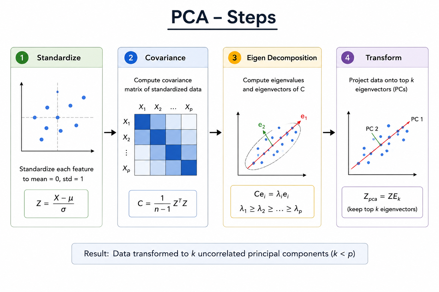
What is Principal Component Analysis (PCA), and what is its purpose?

GoogleAmazonMicrosoftMetaApple

Solution

Principal Component Analysis (PCA) is a dimensionality reduction technique that reduces the number of features while preserving the maximum variance in the data.

How PCA Works:

1. Standardize the data — zero mean, unit variance.

2. Compute the covariance matrix — captures relationships between features.

3. Calculate eigenvalues and eigenvectors of the covariance matrix.

4. Rank components by eigenvalue — higher eigenvalue = more variance explained.

5. Select top k components with the highest eigenvalues.

6. Transform data into the new lower-dimensional feature space.

Key Concepts:

•Principal Components — new orthogonal axes that capture maximum variance.

•Eigenvalues — represent the amount of variance captured by each component.

•Eigenvectors — define the direction of each principal component.

Benefits of PCA:

•Reduces dimensionality — fewer features, simpler models.

•Speeds up training — less data to process.

•Removes multicollinearity — components are orthogonal (uncorrelated).

•Aids visualization — reduce to 2D or 3D for plotting.

•Reduces overfitting — removes noise dimensions.

Example:

•A dataset with 100 features reduced to 10 principal components retaining 95% of variance.

Limitation:

•PCA is a linear technique — may not work well for non-linearly structured data.

•Components are less interpretable than original features.

What is Principal Component Analysis (PCA), and what is its purpose? image 1

Figure 49: ★ Principal Component Analysis (PCA)

What is Reinforcement Learning, and how does it differ from other types of learning?

GoogleAmazonMicrosoftMetaOpenAI

Solution

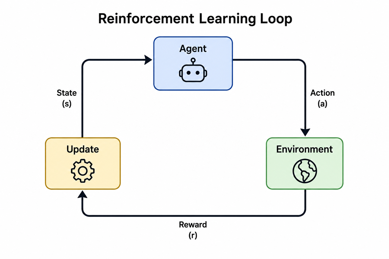
Reinforcement Learning (RL) is a type of machine learning where an agent learns to make decisions by interacting with an environment. The agent receives rewards or penalties based on its actions and seeks to maximize cumulative rewards over time.

Key Components:

•Agent — the learner or decision maker.

•Environment — the world the agent interacts with.

•State (s) — the current situation of the environment.

•Action (a) — the decision taken by the agent.

•Reward (r) — feedback signal received after taking an action.

•Policy (π) — the strategy mapping states to actions.

How RL Works:

1. Agent observes the current state.

2. Agent takes an action based on its policy.

3. Environment returns a new state and reward.

4. Agent updates its policy to maximize future rewards.

Return Formula:

G = Σ γᵗ × Rₜ (summed from t=0 to infinity)

where γ (gamma) = discount factor (0 to 1) and Rₜ = reward at time t.

How RL Differs:

•Supervised Learning — learns from labeled input-output pairs.

•Unsupervised Learning — finds patterns in unlabeled data.

•Reinforcement Learning — learns through trial and error with reward signals — no labeled data needed.

Applications:

•Robotics, Game playing (Chess, Go, Atari), Self-driving cars, Recommendation systems, Resource management.

What is Reinforcement Learning, and how does it differ from other types of learning? image 1

Figure 50: ★ Reinforcement Learning Framework